列と行を1 つの列に転置・変換するには、どうすればよいですか？

著者Xiaoyang変更日2024-08-21

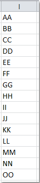
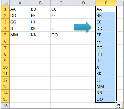
Excel ワークシートを使用していると、次のような問題に直面することがあります。「範囲内のデータを1 つの列に変換または転置するにはどうすればよいでしょうか？」（以下のスクリーンショットを参照）。ここでは、この課題を解決するための3 つの簡単なテクニックをご紹介します。

数式で列と行を1 つの列に転置／変換する

Kutools for Excel で列と行を1 つの列に転置／変換する

VBA コードで列と行を1 つの列に転置／変換する

数式で列と行を1 つの列に転置／変換する

次の長い数式を使えば、データ範囲をすばやく列に転置できます。以下の手順に従ってください。

1。まず、変換したいデータ範囲を選択し、右クリックしてコンテキストメニューから名前の定義を選択します。表示される新しい名前ダイアログボックスで、任意の名前を入力してOKをクリックし、そのデータ範囲にセルの名前を定義します。（スクリーンショットを参照）

データ範囲に名前を定義

2。セルの名前を指定した後、空白セル（この例ではセル E1）をクリックして、次の数式を入力します。=INDEX(MyData,1+INT((ROW(A1)-1)/COLUMNS(MyData)),MOD(ROW(A1)-1+COLUMNS(MyData),COLUMNS(MyData))+1)。

注：MyDataは、データ選択範囲のセル名です。必要に応じて変更できます。

3。その後、エラーが表示されるまで数式を下方向にドラッグしてください。これにより、範囲内のすべてのデータが1 つの列に転置されます。（スクリーンショット参照）

結果を得るために数式を入力

Kutools for Excel で列と行を1 つの列に転置／変換する

数式が長すぎて覚えにくく、VBA コードにも制限がある場合でもご安心ください。ここでは、さらに簡単で多機能なツール——Kutools for Excelをご紹介します。そのTransform Range 機能を使えば、この問題を素早く簡単に解決できます。

Kutools for Excelは300 以上の高度な機能を提供し、複雑な作業を効率化して、創造性と生産性を高めます。AI 機能と統合されたKutools は、正確にタスクを自動化し、データ管理を簡単にします。Kutools for Excel の詳細情報。。。 無料トライアル。。。

無料でインストールした後、以下の手順に従ってください。

1。転置したい範囲を選択します。

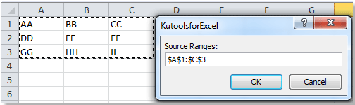
2。Kutools>範囲を変換をクリックします。（スクリーンショットを参照）

Kutools の「範囲の変換」機能をクリック

3。表示されるTransform Rangeダイアログボックスで、Range to single columnオプションを選択してください。（スクリーンショットを参照）

「範囲を1列に」オプションを選択

4。次に、OKをクリックして、ポップアップボックスから結果を出力するセルを指定します。

結果を配置するセルを指定

5。OKをクリックすると、複数の列と行にわたるデータが1 つの列に転置されます。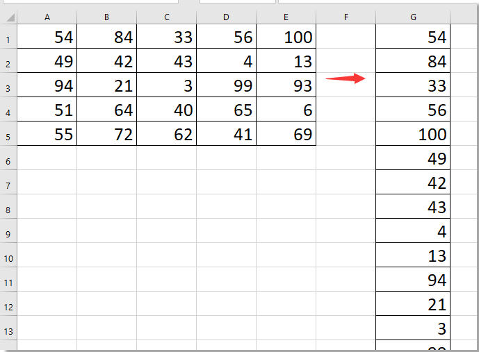
範囲のデータが1列に転置されました

固定値を使って列を範囲に変換したい場合は、Transform Range 機能を使えば、素早く簡単に処理できます！
Kutools を使用して1列を範囲に変換

VBA コードで列と行を1 つの列に転置／変換する

次の VBA コードを使えば、複数の列と行を1 つの列に結合できます。

1。ALT + F11キーを押して、Microsoft Visual Basic for Applicationsウィンドウを開きます。

2。挿入 > モジュールをクリックし、表示されるモジュールウィンドウに次のコードを貼り付けてください。

Sub ConvertRangeToColumn()
'Updateby20131126
Dim Range1 As Range, Range2 As Range, Rng As Range
Dim rowIndex As Integer
xTitleId = "KutoolsforExcel"
Set Range1 = Application.Selection
Set Range1 = Application.InputBox("Source Ranges:", xTitleId, Range1.Address, Type:=8)
Set Range2 = Application.InputBox("Convert to (single cell):", xTitleId, Type:=8)
rowIndex = 0
Application.ScreenUpdating = False
For Each Rng In Range1.Rows
    Rng.Copy
    Range2.Offset(rowIndex, 0).PasteSpecial Paste:=xlPasteAll, Transpose:=True
    rowIndex = rowIndex + Rng.Columns.Count
Next
Application.CutCopyMode = False
Application.ScreenUpdating = True
End Sub

3。F5キーを押してコードを実行すると、変換する範囲を選択するダイアログが表示されます。（スクリーンショットを参照）

データ範囲を選択する VBA コード

4。次にOKをクリックすると、結果を出力するセルを1 つ選択するための別のダイアログが表示されます。（スクリーンショットを参照）

結果を配置するセルを選択する VBA コード

5。OKをクリックすると、指定範囲のセル内容が1 つの列にリスト形式で変換されます。（スクリーンショットを参照）

結果を得るための VBA コード

関連記事：

Excel で行を列に変更する方法は？

Excel で1 つの列を複数の列に転置または変換するには、どうすればよいですか？

列と行を1 つの行に転置／変換するには、どうすればよいですか？

最高の Office 業務効率化ツール

🤖	KUTOOLS AI アシスタント：次に基づいてデータ分析を革新します：インテリジェント実行｜コード生成｜カスタム数式作成｜データ分析とチャート生成｜拡張機能呼び出し…
	人気の機能：検索・ハイライト、または重複をマーキング｜空白行を削除する｜データを失うことなく列の結合またはセルを｜数式を使用しない四捨五入...
	スーパー LOOKUP：複数条件 VLookup ｜複数値 VLookup ｜複数シート間 VLookup ｜ファジーマッチ....
	高度なドロップダウンリスト：ドロップダウンリストをすばやく作成｜連動型ドロップダウンリスト｜複数選択可能なドロップダウンリスト....
	列マネージャー：指定した数の列を追加｜列の移動｜非表示列の表示状態を切り替え｜範囲および列の比較...
	注目の機能：グリッドフォーカス｜デザインビュー｜強化された数式バー｜ワークブックとシートマネージャー｜リソースライブラリ（オートテキスト）｜日付ピッカー｜ワークシートの統合｜暗号化／セルの復号化｜リストからメール送信｜スーパーフィルター｜特殊フィルタ（太字のフォントを持つセルをフィルタリング／斜体／取り消し線。。。）。。。
	トップ15 ツールセット：12 テキストツール（テキストの追加、特定の文字を削除、...）｜ 50+チャートタイプ（ガントチャート、...）｜ 40+実用的関数（誕生日に基づいて年齢を計算します、...）｜ 19 挿入ツール（QR コードを挿入、パスから画像を挿入、...）｜ 12 変換ツール（単語に変換する、為替レートの変換、...）｜ 7 結合と分割ツール（高度な行のマージ、セルの分割、...）｜さらに多数

Kutools はお好みの言語でご利用いただけます。英語、スペイン語、ドイツ語、フランス語、中国語、および40+の他の言語をサポートしています！

Kutools for Excel でExcel スキルを強化し、これまでにない効率を体験しましょう。Kutools for Excel は、生産性を高め、時間を大幅に節約できる高度な機能を300 以上提供します。最も必要な機能を今すぐ入手するにはこちらをクリック。。。

Kutools for Excel の詳細はこちら。。。無料ダウンロード。。。

Office Tab は Office にタブインターフェースをもたらし、作業を大幅に簡単にします

Word、Excel、PowerPoint でタブを使った編集と閲覧を有効にします。Publisher、Access、Visio、Project でもご利用いただけます。
複数のドキュメントを、新しいウィンドウではなく、同じウィンドウ内の新しいタブで開いたり作成したりできます。
日々の生産性を50％も向上させ、毎日数百回ものマウスクリックを削減します！

Office Tab の詳細はこちら。。。無料ダウンロード。。。

すべてのKutools アドインが、たった1 つのインストーラーで完結。

Kutools for Officeスイートには、Excel ・Word ・Outlook ・PowerPoint 用のアドインと Office Tab Pro が含まれており、複数の Office アプリを横断して作業するチームに最適です。

オールインワンスイート— Excel、Word、Outlook、PowerPoint 用アドイン＋Office Tab Pro
インストーラー1 つ、ライセンス1 つ— 数分でセットアップ可能（MSI 対応）
連携してさらにパワーアップ— Office アプリ全体で生産性が向上
30 日間のフル機能トライアル— 登録不要、クレジットカード不要
最高のお得感— 個別アドイン購入よりお得

Kutools for Office の詳細はこちら。。。無料ダウンロード。。。