Excelでフィルターされたセルまたは表示されているセルのみを合計するにはどうすればよいですか?
Excelで列の数字を合計するのは簡単かもしれませんが、時には基準に合うようにデータをフィルタリングしたり非表示にしたりする必要があります。隠したりフィルタリングした後、フィルタリングされた値や表示されている値だけを合計したい場合があります。ExcelでSum関数を使用すると、隠されたデータも含めてすべての値が加算されてしまいます。このような場合、Excelでフィルタリングされたセルや表示されているセルの値のみを合計するにはどうすればよいでしょうか?
- 数式を使ってフィルタリングされたセルや表示されているセルの値のみを合計する
- ユーザー定義関数を使用してフィルタリングされたセルや表示されているセルの値のみを合計する
- Kutools for Excelを使用してフィルタリングされたセルや表示されているセルのみを合計/カウント/平均する
数式を使ってフィルタリングされたセルや表示されているセルの値のみを合計する
フィルタによって除外された行を無視するSUBTOTAL関数を使用することで、表示されているセルのみを簡単に合計できます。以下のように操作します:
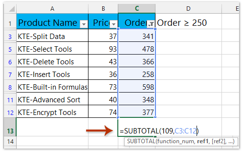
範囲のデータがあり、必要なようにすでにフィルタリングされていると仮定します。スクリーンショットをご覧ください:

1空白のセル(例:C13)に次の数式を入力します: =Subtotal(109,C2:C12) (109 これは、合計する際に隠された値は無視されることを示しています; C2:C12 は、フィルタリングされた行を無視して合計する範囲です。そして、「Enter」キーを押します。 Enter キーを押します。
注: この数式は、ワークシートに隠し行がある場合にも表示されているセルのみを合計するのに役立ちます。ただし、この数式では隠し列内のセルを無視して合計することはできません。
隠しセル、行、または列を無視して指定された範囲内の表示されているセルのみを合計/カウント/平均する
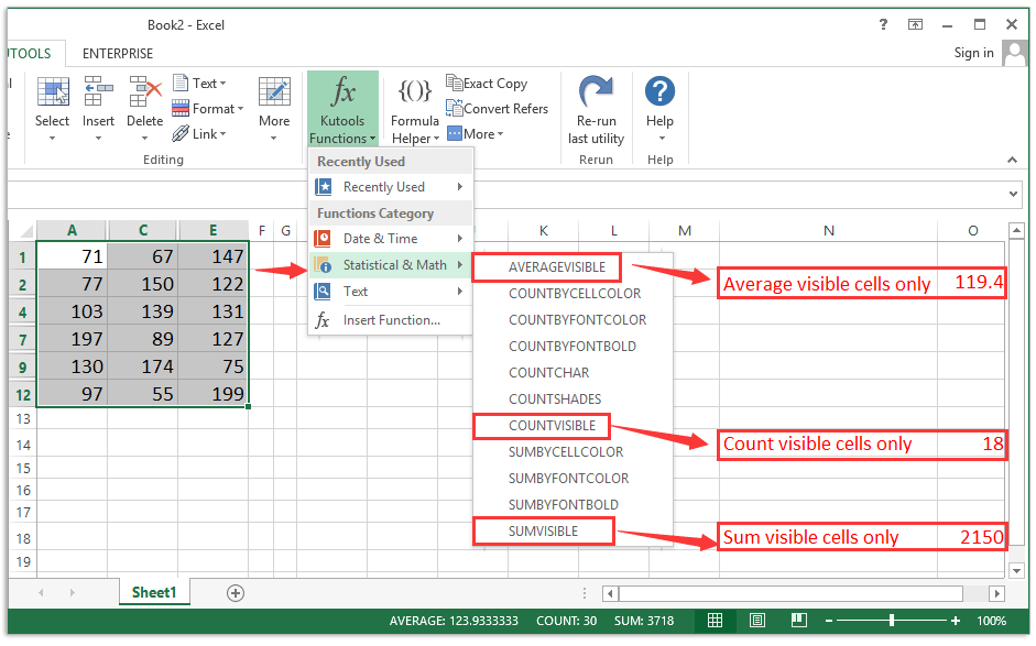
通常のSUM/Count/Average関数は、セルが隠されているかフィルタリングされているかに関係なく、指定された範囲内のすべてのセルをカウントします。一方、Subtotal関数は隠し行を無視して合計/カウント/平均することができます。しかし、Kutools for Excelの SUMVISIBLE / COUNTVISIBLE / AVERAGEVISIBLE 関数は、隠しセル、行、または列を無視して指定された範囲を簡単に計算します。
ユーザー定義関数を使用してフィルタリングされたセルや表示されているセルの値のみを合計する
以下のコードに興味がある場合、これも表示されているセルのみを合計するのに役立ちます。
1. ALT + F11キーを押すと、Microsoft Visual Basic for Applicationsウィンドウが開きます。
2. 「 挿入」>「モジュール」をクリックし、モジュールウィンドウに次のコードを貼り付けます。
Function SumVisible(WorkRng As Range) As Double
'Update 20130907
Dim rng As Range
Dim total As Double
For Each rng In WorkRng
    If rng.Rows.Hidden = False And rng.Columns.Hidden = False Then
        total = total + rng.Value
    End If
Next
SumVisible = total
End Function
3このコードを保存し、数式を入力します =SumVisible(C2:C12) 空白のセルに入力します。スクリーンショットをご覧ください:

4. その後、「 Enter」キーを押すと、求めている結果が得られます。
Kutools for Excelを使用してフィルタリングされたセルや表示されているセルのみを合計/カウント/平均する
Kutools for Excelがインストールされている場合、Excelで表示されているセルまたはフィルタリングされたセルのみを簡単に合計/カウント/平均できます。
Kutools for Excel - 必要なツールを300以上搭載し、Excelの機能を大幅に強化します。永久に無料で利用できるAI機能もお楽しみください!今すぐ入手
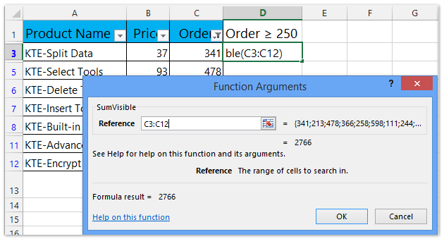
たとえば、表示されているセルのみを合計したい場合、合計結果を配置するセルを選択し、数式 =SUMVISIBLE(C3:C12) (C3:C13は表示されているセルのみを合計する範囲)を入力し、「Enter」キーを押します。
そして、すべての隠しセルを無視して合計結果が計算されます。スクリーンショットをご覧ください:

表示されているセルのみをカウントするには、この数式 =COUNTVISIBLE(C3:C12) を使用してください。表示されているセルのみを平均するには、この数式 =AVERAGEVISIBLE(C3:C12) を使用してください。
注: 数式を正確に覚えていない場合は、以下の手順に従って表示されているセルのみを簡単に合計/カウント/平均できます:
1. 合計結果を配置するセルを選択し、 Kutools > 関数 > 数学 & 統計 > SUMVISIBLE (または AVERAGEVISBLE, COUNTVISIBLE 必要に応じて選択)。スクリーンショットをご覧ください:

2. 開いた「関数の引数」ダイアログボックスで、隠しセルを無視して合計する範囲を指定し、「OK 」ボタンをクリックします。スクリーンショットをご覧ください:
Kutools for Excel - 必要なツールを300以上搭載し、Excelの機能を大幅に強化します。永久に無料で利用できるAI機能もお楽しみください!今すぐ入手
そして、すべての隠しセルを無視して合計結果が計算されます。
関連記事:
最高のオフィス業務効率化ツール
| 🤖 | Kutools AI Aide:データ分析を革新します。主な機能:Intelligent Execution|コード生成|カスタム数式の作成|データの分析とグラフの生成|Kutools Functionsの呼び出し…… |
| 人気の機能:重複の検索・ハイライト・重複をマーキング|空白行を削除|データを失わずに列またはセルを統合|丸める…… | |
| スーパーLOOKUP:複数条件でのVLookup|複数値でのVLookup|複数シートの検索|ファジーマッチ…… | |
| 高度なドロップダウンリスト:ドロップダウンリストを素早く作成|連動ドロップダウンリスト|複数選択ドロップダウンリスト…… | |
| 列マネージャー:指定した数の列を追加 |列の移動 |非表示列の表示/非表示の切替| 範囲&列の比較…… | |
| 注目の機能:グリッドフォーカス|デザインビュー|強化された数式バー|ワークブック&ワークシートの管理|オートテキスト ライブラリ|日付ピッカー|データの統合 |セルの暗号化/復号化|リストで電子メールを送信|スーパーフィルター|特殊フィルタ(太字/斜体/取り消し線などをフィルター)…… | |
| トップ15ツールセット:12 種類のテキストツール(テキストの追加、特定の文字を削除など)|50種類以上のグラフ(ガントチャートなど)|40種類以上の便利な数式(誕生日に基づいて年齢を計算するなど)|19 種類の挿入ツール(QRコードの挿入、パスから画像の挿入など)|12 種類の変換ツール(単語に変換する、通貨変換など)|7種の統合&分割ツール(高度な行のマージ、セルの分割など)|… その他多数 |
Kutools for ExcelでExcelスキルを強化し、これまでにない効率を体感しましょう。 Kutools for Excelは300以上の高度な機能で生産性向上と保存時間を実現します。最も必要な機能はこちらをクリック...
Office TabでOfficeにタブインターフェースを追加し、作業をもっと簡単に
- Word、Excel、PowerPointでタブによる編集・閲覧を実現。
- 新しいウィンドウを開かず、同じウィンドウの新しいタブで複数のドキュメントを開いたり作成できます。
- 生産性が50%向上し、毎日のマウスクリック数を何百回も削減!
全てのKutoolsアドインを一つのインストーラーで
Kutools for Officeスイートは、Excel、Word、Outlook、PowerPoint用アドインとOffice Tab Proをまとめて提供。Officeアプリを横断して働くチームに最適です。
- オールインワンスイート — Excel、Word、Outlook、PowerPoint用アドインとOffice Tab Proが含まれます
- 1つのインストーラー・1つのライセンス —— 数分でセットアップ完了(MSI対応)
- 一括管理でより効率的 —— Officeアプリ間で快適な生産性を発揮
- 30日間フル機能お試し —— 登録やクレジットカード不要
- コストパフォーマンス最適 —— 個別購入よりお得