Excelでアクティブな行と列を自動的にハイライトする(完全ガイド)
膨大なデータが詰まったExcelワークシートをナビゲートするのは難しい場合があり、場所を見失ったり値を読み間違えたりしやすいです。データ分析を強化し、エラーの可能性を減らすために、ここではExcelで選択したセルの行と列を動的にハイライトする3つの異なる方法を紹介します。セルからセルへ移動すると、ハイライトも動的に切り替わり、次のデモのように正しいデータに集中できる明確で直感的な視覚的な手がかりを提供します:
Excelでアクティブな行と列を自動的にハイライトする
- VBAコードを使用 - 既存のセルの色をクリアし、元に戻す(Undo)はサポートされません
- Kutools for Excelをワンクリック - 既存のセルの色を保持し、元に戻す(Undo)をサポート、保護されたシートにも適用可能
- 条件付き書式を使用 - 大量のデータでは不安定、手動での更新(F9)が必要
VBAコードでアクティブな行と列を自動的にハイライトする
現在のワークシートで選択したセルの列と行全体を自動的にハイライトするには、以下のVBAコードがこのタスクを達成するのに役立つかもしれません。
ステップ1: 自動的にアクティブな行と列をハイライトしたいワークシートを開きます
ステップ2: VBAシートモジュールエディターを開き、コードをコピーします
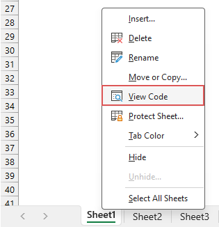
- シート名を右クリックし、コンテキストメニューから「コードの表示」を選択します。スクリーンショットをご覧ください:
- 開かれたVBAシートモジュールエディターで、以下のコードを空白のモジュールにコピーして貼り付けます。スクリーンショットをご覧ください:
VBAコード: 選択したセルの行と列を自動的にハイライトするPrivate Sub Worksheet_SelectionChange(ByVal Target As Range) 'Update by Extendoffice Dim rowRange As Range Dim colRange As Range Dim activeCell As Range Set activeCell = Target.Cells(1, 1) Set rowRange = Rows(activeCell.Row) Set colRange = Columns(activeCell.Column) Cells.Interior.ColorIndex = xlNone rowRange.Interior.Color = RGB(248, 150, 171) colRange.Interior.Color = RGB(173, 233, 249) End Subヒント: コードのカスタマイズ- ハイライトの色を変更するには、以下のスクリプト内のRGB値を修正するだけです:
rowRange.Interior.Color = RGB(248, 150, 171)
colRange.Interior.Color = RGB(173, 233, 249) - 選択したセルの行全体のみをハイライトするには、この行を削除するかコメントアウト(先頭にアポストロフィを追加)します:
colRange.Interior.Color = RGB(173, 233, 249) - 選択したセルの列全体のみをハイライトするには、この行を削除するかコメントアウト(先頭にアポストロフィを追加)します:
rowRange.Interior.Color = RGB(248, 150, 171)

- ハイライトの色を変更するには、以下のスクリプト内のRGB値を修正するだけです:
- その後、VBAエディターウィンドウを閉じてワークシートに戻ります。


結果:
これで、セルを選択するとそのセルの行と列全体が自動的にハイライトされ、選択したセルが変わるとハイライトも動的に切り替わります。以下のようなデモをご覧ください:
- このコードはワークシート内のすべてのセルの背景色をクリアするため、カスタムカラーが設定されているセルがある場合はこの解決策を使用しないでください。
- このコードを実行すると、シートの「元に戻す(Undo)」機能が無効になり、「Ctrl」+「Z」のショートカットでミスを元に戻すことができなくなります。
- このコードは保護されたワークシートでは動作しません。
- 選択したセルの行と列のハイライトを停止するには、以前に追加したVBAコードを削除する必要があります。その後、「ホーム」>「塗りつぶしの色」>「塗りつぶしなし」をクリックしてハイライトをリセットします。
Kutoolsの一回のクリックでアクティブな行と列を自動的にハイライトする
ExcelのVBAコードの限界に直面していますか?「Kutools for Excel」の「グリッドフォーカス」機能は理想的なソリューションです!VBAの欠点に対処するために設計されており、シート体験を向上させる多様なハイライトスタイルを提供します。「Kutools」はこれらのスタイルをすべての開いているワークブックに適用でき、一貫して効率的で視覚的に魅力的なデータ管理プロセスを確保します。
Kutools for Excelをインストール後、「Kutools」>「グリッドフォーカス」をクリックしてこの機能を有効にします。これで、アクティブなセルの行と列がすぐにハイライトされます。このハイライトは、セルの選択が変わるたびに動的に移動します。以下のデモをご覧ください:
- 元のセルの背景色を保持:
VBAコードとは異なり、この機能はワークシートの既存の書式設定を尊重します。 - 保護されたシートでも使用可能:
この機能は保護されたワークシートでもシームレスに動作し、セキュリティを損なうことなく機密または共有ドキュメントを管理するのに最適です。 - 元に戻す機能に影響を与えない:
この機能を使用すると、Excelの元に戻す機能にフルアクセスできます。これにより、データ操作に安全層を追加しつつ、簡単に変更を元に戻すことができます。 - 大量のデータでも安定したパフォーマンス:
この機能は大量のデータセットを効率的に処理するように設計されており、複雑でデータ集約的なスプレッドシートでも安定したパフォーマンスを確保します。 - 複数のハイライトスタイル:
この機能はさまざまなハイライトオプションを提供し、行、列、または行と列のアクティブなセルを目立たせるスタイルや色を選択できます。これにより、好みやニーズに最も適した形でデータを強調できます。

- この機能を無効にするには、「Kutools」>「グリッドフォーカス」を再度クリックしてこの機能を閉じてください;
- この機能を適用するには、Kutools for Excelをダウンロードしてインストールしてください。
条件付き書式を使用してアクティブな行と列を自動的にハイライトする
Excelでは、条件付き書式を設定してアクティブな行と列を自動的にハイライトすることもできます。この機能を設定するには、次の手順に従ってください:
ステップ1: データ範囲を選択
まず、この機能を適用したいセルの範囲を選択します。これはワークシート全体でも特定のデータセットでもかまいません。ここでは、ワークシート全体を選択します。
ステップ2: 条件付き書式にアクセス
「ホーム」>「条件付き書式」>「新しいルール」をクリックします。スクリーンショットをご覧ください:
ステップ3: 新しい書式ルールで操作を設定
- 「新しい書式ルール」ダイアログボックスで、「ルールの種類を選択」リストボックスから「数式を使用して書式設定するセルを決定」を選択します。
- 「この数式が真の場合に値を書式設定」ボックスに、以下の数式のいずれかを入力します。この例では、アクティブな行と列をハイライトするために3番目の数式を適用します。
アクティブな行をハイライトするには:
アクティブな列をハイライトするには:=CELL("row")=ROW()
アクティブな行と列をハイライトするには:=CELL("col")=COLUMN()=OR(CELL("row")=ROW(), CELL("col")= COLUMN()) - 次に、「書式」ボタンをクリックします。

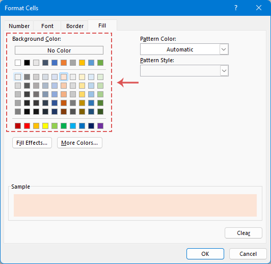
- 続く「セルの書式設定」ダイアログボックスで、「塗りつぶし」タブの下で、必要に応じてアクティブな行と列をハイライトする色を選択します。スクリーンショットをご覧ください:
- 次に、「OK」>「OK」をクリックしてダイアログを閉じます。


結果:
これで、セルA1の列と行全体が一度にハイライトされているのがわかります。このハイライトを別のセルに適用するには、目的のセルをクリックして「F9」キーを押してシートを更新するだけで、新しく選択したセルの列と行全体がハイライトされます。
- 確かに、Excelでの条件付き書式によるハイライト方法は解決策を提供しますが、「VBA」と「グリッドフォーカス」機能ほどシームレスではありません。この方法では、シートの手動再計算が必要です(「F9」キーを押すことで実現)。
ワークシートの自動再計算を有効にするには、ターゲットシートのコードモジュールに簡単なVBAコードを組み込むことができます。これにより、異なるセルを選択するたびに「F9」キーを押さなくてもハイライトが即座に更新されるようになります。シート名を右クリックし、コンテキストメニューから「コードの表示」を選択します。その後、次のコードをシートモジュールにコピーして貼り付けてください:Private Sub Worksheet_SelectionChange(ByVal Target As Range) Target.Calculate End Sub - 条件付き書式は、ワークシートに手動で適用した既存の書式設定を保持します。
- 条件付き書式は揮発性が高いことが知られており、特に非常に大きなデータセットに適用すると、ワークブックのパフォーマンスが低下する可能性があります。これにより、データ処理やナビゲーションの効率に影響を与えることがあります。
- CELL関数はExcel 2007以降のバージョンでのみ利用可能です。この方法はそれ以前のバージョンのExcelでは互換性がありません。
上記の方法の比較
| 機能 | VBAコード | 条件付き書式 | Kutools for Excel |
| セルの背景色を保持 | いいえ | はい | はい |
| 元に戻す(Undo)をサポート | いいえ | はい | はい |
| 大量のデータセットで安定 | いいえ | いいえ | はい |
| 保護されたシートで使用可能 | いいえ | はい | はい |
| すべての開いているワークブックに適用 | 現在のシートのみ | 現在のシートのみ | すべての開いているワークブック |
| 手動での更新(F9)が必要 | いいえ | はい | いいえ |
以上で、Excelで選択したセルの列と行をハイライトする方法に関するガイドを終了します。さらに多くのExcelのヒントやコツに興味がある場合、当サイトには数千のチュートリアルがありますので、 こちらをクリックしてアクセスしてください。ご閲覧いただきありがとうございます。今後も役立つ情報を提供できることを楽しみにしています!
関連記事:
- アクティブなセルの行と列を自動的にハイライトする
- 多数のデータを持つ大規模なワークシートを表示しているとき、選択したセルの行と列をハイライトして、データを誤読しないように簡単に直感的に読めるようにしたい場合があります。ここでは、現在のセルの行と列をハイライトするいくつかの興味深いトリックを紹介します。セルが変更されると、新しいセルの列と行が自動的にハイライトされます。
- Excelで交互に行または列をハイライトする
- 大規模なワークシートでは、交互またはn行ごとに行または列をハイライトまたは塗りつぶすことで、データの可視性と読みやすさが向上します。ワークシートがより整然として見えるだけでなく、データをより迅速に理解するのに役立ちます。この記事では、データをより魅力的で分かりやすく提示するための、交互またはn行ごとの行または列をシェードするさまざまな方法を説明します。
- スクロール中に行全体をハイライトする
- 複数の列を持つ大規模なワークシートがある場合、その行のデータを区別するのが難しくなることがあります。このような場合、アクティブなセルの行全体をハイライトすることで、水平スクロールバーをスクロールダウンしてもその行のデータを素早く簡単に確認できます。この記事では、この問題を解決するためのいくつかのトリックについて説明します。
- ドロップダウンリストに基づいて行をハイライトする
- この記事では、ドロップダウンリストに基づいて行をハイライトする方法について説明します。次のスクリーンショットを例に取ると、列Eのドロップダウンリストから「進行中」を選択すると、その行が赤色でハイライトされ、「完了」を選択すると青色でハイライトされ、「未開始」を選択すると緑色でハイライトされます。
最高のオフィス業務効率化ツール
| 🤖 | Kutools AI Aide:データ分析を革新します。主な機能:Intelligent Execution|コード生成|カスタム数式の作成|データの分析とグラフの生成|Kutools Functionsの呼び出し…… |
| 人気の機能:重複の検索・ハイライト・重複をマーキング|空白行を削除|データを失わずに列またはセルを統合|丸める…… | |
| スーパーLOOKUP:複数条件でのVLookup|複数値でのVLookup|複数シートの検索|ファジーマッチ…… | |
| 高度なドロップダウンリスト:ドロップダウンリストを素早く作成|連動ドロップダウンリスト|複数選択ドロップダウンリスト…… | |
| 列マネージャー:指定した数の列を追加 |列の移動 |非表示列の表示/非表示の切替| 範囲&列の比較…… | |
| 注目の機能:グリッドフォーカス|デザインビュー|強化された数式バー|ワークブック&ワークシートの管理|オートテキスト ライブラリ|日付ピッカー|データの統合 |セルの暗号化/復号化|リストで電子メールを送信|スーパーフィルター|特殊フィルタ(太字/斜体/取り消し線などをフィルター)…… | |
| トップ15ツールセット:12 種類のテキストツール(テキストの追加、特定の文字を削除など)|50種類以上のグラフ(ガントチャートなど)|40種類以上の便利な数式(誕生日に基づいて年齢を計算するなど)|19 種類の挿入ツール(QRコードの挿入、パスから画像の挿入など)|12 種類の変換ツール(単語に変換する、通貨変換など)|7種の統合&分割ツール(高度な行のマージ、セルの分割など)|… その他多数 |
Kutools for ExcelでExcelスキルを強化し、これまでにない効率を体感しましょう。 Kutools for Excelは300以上の高度な機能で生産性向上と保存時間を実現します。最も必要な機能はこちらをクリック...
Office TabでOfficeにタブインターフェースを追加し、作業をもっと簡単に
- Word、Excel、PowerPointでタブによる編集・閲覧を実現。
- 新しいウィンドウを開かず、同じウィンドウの新しいタブで複数のドキュメントを開いたり作成できます。
- 生産性が50%向上し、毎日のマウスクリック数を何百回も削減!
全てのKutoolsアドインを一つのインストーラーで
Kutools for Officeスイートは、Excel、Word、Outlook、PowerPoint用アドインとOffice Tab Proをまとめて提供。Officeアプリを横断して働くチームに最適です。
- オールインワンスイート — Excel、Word、Outlook、PowerPoint用アドインとOffice Tab Proが含まれます
- 1つのインストーラー・1つのライセンス —— 数分でセットアップ完了(MSI対応)
- 一括管理でより効率的 —— Officeアプリ間で快適な生産性を発揮
- 30日間フル機能お試し —— 登録やクレジットカード不要
- コストパフォーマンス最適 —— 個別購入よりお得