Excel で複数の列から一意の値を抽出するには、どうすればよいですか？

著者Xiaoyang変更日2025-07-14

Excel で複数の列にまたがるデータセットを頻繁に扱う際、同じ列内や異なる列間で特定の値が重複していることに気づくことは珍しくありません。多くのレポート作成やデータ分析タスクでは、選択範囲全体において一度しか出現しない一意の値（その位置にかかわらず）を特定・抽出する必要があります。これを手動で行うと、特に大規模なデータセットや複雑な表を扱う場合、時間もかかりミスも起こりやすくなります。幸いにも、Excel にはこうした一意の値を効率的に抽出するためのさまざまな方法が用意されています。

このガイドでは、お使いのExcel バージョンや目的に応じて選べるさまざまな解決策をご紹介します。具体的には、すべてのバージョンで使える標準の数式、最新バージョン向けの動的配列数式、手軽に結果を得られる KUTOOLS AI Aide、データを視覚的に統合するピボットテーブル、そして複雑なシナリオで自動抽出を行う VBA コードなどが含まれます。

数式を使用して複数列から一意の値を抽出する
- 配列数式（すべてのExcel バージョン）
- 数式（Excel 365、Excel 2021、およびそれ以降のバージョン）
KUTOOLS AI Aide を使用して複数列から一意の値を抽出する
PivotTable を使用して複数列から一意の値を抽出する
VBA コードを使用して複数列から一意の値を抽出する

数式を使用して複数列から一意の値を抽出する

組み込みのExcel 関数を使ってこの抽出を実現したいと思うこともあるでしょう。本セクションでは、すべてのExcel バージョンで使える配列数式と、Excel 365 やExcel 2021 など最新バージョンで利用可能な動的配列数式という2 つのアプローチを詳しく解説します。これらの方法は、数式ベースのソリューションを直接使いたいとき、データ変更時に頻繁に更新が必要なとき、または外部アドインやコードを使いたくないときに最適です。

すべてのExcel バージョンで使用可能な配列数式で複数列から一意の値を抽出する

すべてのExcel バージョンとの互換性を確保するには、配列数式を使って複数列から一意の値を抽出できます。これにより、動的配列をサポートしていないExcel でも問題なく動作します。このアプローチでは、INDIRECT、TEXT、MIN、IF、COUNTIF、ROW、COLUMN 関数を組み合わせることで、さまざまなデータ構造にも柔軟に対応可能です。

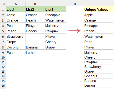
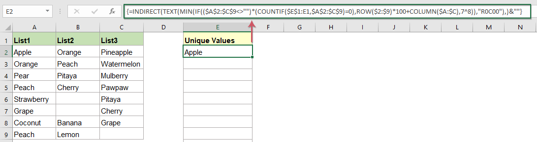
データがA2:C9の範囲にあると仮定します。セルE2から一意の値を抽出するには、次の手順に従ってください：

1。セルE2（またはリスト配置エリアの先頭セル）をクリックし、次の配列数式を入力してください：

=INDIRECT(TEXT(MIN(IF(($A$2:$C$9<>「」)*(COUNTIF($E$1:E1,$A$2:$C$9)=0),ROW($2:$9)*100+COLUMN($A:$C),7^8)),"R0C00"),)&「」

注：この数式について：

A2:C9は、一意の値を抽出したいデータ範囲です。
E1:E1は、最初の出力セルの直上にあるセルを指し、すでに抽出されたエントリを追跡するために必要です。
$2:$9はデータの行範囲を示し、$A:$Cは列範囲を示します。ワークシートのレイアウトに合わせて、必要に応じて調整してください。

実際のデータが別の場所にある場合は、必ず範囲を更新してください。

Excelで配列数式を使用して一意の値を抽出する方法を示すスクリーンショット

2。数式を入力したら、Enter キーを押すのではなく、Ctrl + Shift + Enterを同時に押して、配列数式として確定してください。正しく実行されると、数式バーに数式の両側に波括弧｛｝が表示されます。その後、E2から下方向へフィルハンドルをドラッグします。空白セルが現れるまでドラッグし続けると、抽出すべき一意の値がすべて表示されたことを示します。この操作により、対象列にすべての一意な値が表示されます。

Excelで配列数式を使用して抽出された一意の値を示すスクリーンショット

この数式の説明：

$A$2:$C$9：一意の値を検索する対象として、セルの全体を指定します。
IF(($A$2:$C$9<>「」)*(COUNTIF($E$1:E1,$A$2:$C$9)=0), ROW($2:$9)*100+COLUMN($A:$C),7^8):
- $A$2:$C$9<>「」は、空白セルを確実に無視します。
- COUNTIF($E$1:E1,$A$2:$C$9)=0は、新規（まだ抽出されていない）値のみを含むようにします。
- 両方の条件が満たされると、セルの行と列に基づいた計算により対応する出力が生成され、一意のインデックス番号が得られます。
- いずれかの条件が満たされない場合、数式が誤って選択されないように、非常に大きな数（)7^8）を返します。
MIN(...)最小のインデックス番号を特定し、データ内で次に利用可能な一意の値の位置を効果的に見つけ出します。
TEXT(...,"R0C00")R1C1 スタイルを使用して、上記で生成されたインデックスを有効なセル参照に変換します。
INDIRECT(...)上記で作成されたセル参照を、データ範囲内の値に変換します。
&「」数式の結果をテキストとして強制的に処理し、書式設定に起因する予期せぬ問題を回避します。

この方法はすべての Excel バージョンで動作します。ただし、配列数式を正しく使用するには（)Ctrl + Shift + Enter）、そうでないと期待通りの結果が得られない場合があります。また、大規模なデータセットでは配列数式が計算速度を低下させる可能性があるため、中程度のサイズのテーブルで使用するのがパフォーマンス面で最適です。

Excel 365、Excel 2021、およびそれ以降のバージョンで数式を使用して複数列から一意の値を抽出する

Excel 365、Excel 2021、またはそれ以降のバージョンをご利用であれば、動的配列関数を使って、複数列から一意の値を抽出するよりシンプルで直感的な方法が利用できます。UNIQUE 関数とTOCOL 関数を組み合わせれば、複数列にわたるデータを簡単に結合し、たった1 ステップで重複を削除可能。常に更新されるデータや大規模なデータセットを扱う際に特に役立ちます！

この方法を使用するには、空白セル（例：E2、または結果を表示したい任意の場所）を選択し、次の数式を入力してEnterキーを押します：

=UNIQUE(TOCOL(A2:C9,1))

Enter キーを押すと、範囲 A2:C9 内のすべての一意な値が、数式の下のセルに自動的に展開されます。この機能は非常に効率的で、ソースデータが変更されると出力がリアルタイムで自動更新されるため、手動での再読み込み作業が一切不要です。

ExcelのUNIQUE関数が複数の列から一意の値を抽出している様子を示すスクリーンショット

パラメーターの説明：

TOCOL(A2:C9,1)：複数列にわたる値を1 列にすっきり変換し、空白セルは自動で除外します。
UNIQUE(.。。)：各値を1 回だけ抽出し、重複のないクリーンなリストを実現します。

ヒント：データセットが今後変更される可能性がある場合は、この動的ソリューションを使用することで、常に最新の一意のエントリ一覧を維持できます。この方法は Microsoft 365、2021 以降のバージョンでのみ利用可能です。古いバージョンをお使いの場合は、上記の配列数式をご参照ください。

#SPILL！エラーが発生した場合は、結合済みや既存のデータがリスト配置エリアをブロックしていないか確認してください。動的配列は、すべての結果を表示するために数式セルの下に空きスペースが必要です。

KUTOOLS AI Aide を使用して複数列から一意の値を抽出

手作業を減らしてより効率的な方法をお探しですか？Kutools for Excel の「KUTOOLS AI Aide」なら、複数列から簡単に一意の値を抽出できます。数式に不慣れな方や、数式エラーのリスクを避けたい方に特にぴったりです。KUTOOLS AI Aide はあなたの指示を的確に解釈し、データを自動で処理。初心者の方はもちろん、わずか数回のクリックで素早く結果を得たい上級者の方にも最適なソリューションです。

注：KUTOOLS AI Aideを体験するには、必ずKutools for Excel をダウンロードしてインストールしてください。Kutools は使いやすく、幅広い自動化機能を備えたアドインです。

インストール後、KUTOOLS AI > AI アシスタントをクリックして、「KUTOOLS AI Aide」ペインを開きます。

チャットボックスに次のようなリクエストを入力します：「範囲 A2:C9 から空白セルを無視して一意の値を抽出し、結果を E2 から開始してください：」
「送信」をクリックするか Enter キーを押すと、AI がリクエストを分析します。その後、「実行」をクリックするだけで処理が即座に実行され、結果はワークシートの指定位置に表示されます。

ヒント：このソリューションは、データ抽出のワークフローが頻繁に変更される場合や、自然言語処理機能を使いたい場合に特に便利です。元データに空白セルが含まれている可能性がある場合は、AI によるリクエスト内容によって空白エントリが含まれたりフィルターされたりすることがあるため、必ず抽出されたリストを確認してください。

Kutools AI AideがExcelの複数の列から一意の値を抽出する様子を示すGIF

Kutools for Excelは300 以上の高度な機能を提供し、複雑な作業を効率化して、創造性と生産性を高めます。AI 機能と統合されたKutools は、正確にタスクを自動化し、データ管理を簡単にします。Kutools for Excel の詳細情報。。。 無料トライアル。。。

PivotTable を使用して複数列から一意の値を抽出

ピボットテーブルは、視覚的な操作を好む方や、一意の項目を集計したり出現回数をカウントするなど、さらに深く分析したい場合に便利です。この方法は簡単で、数式を一切使う必要がありません。ただし、関連する列の見出しが異なるなどのケースでは、いくつかの設定ステップと多少のデータ再構成が必要になります。

ピボットテーブルを使用して一意の値を抽出する推奨手順は次のとおりです。

1。データのすぐ左側に新しい空白列を挿入します。たとえば、データが列 B から始まる場合は、列 A に新しい列を挿入します。この調整により、範囲の統合が正しく行われるようになります。

Excelでピボットテーブルを使用する前に空白列を追加している様子を示すスクリーンショット

2。データセット内の任意のセルを選択し、Alt + Dを押してからすぐにPを押すと、「ピボットテーブルとピボットグラフレポートウィザード」が起動します。ウィザードの最初のステップで「複数の統合範囲」を選択すると、複数の列にある値を単一の集計フィールドにまとめることが可能になります。

「複数の統合範囲」が選択されているピボットテーブルおよびピボットグラフウィザードのスクリーンショット

3。次へをクリックし、「1 つのページフィールドを作成する」を選択します。これにより、すべてのデータが一意の値を抽出するために単一のグループとして整理されます。

ピボットテーブルウィザードで「単一のページフィールドを作成する」が選択されている様子を示すスクリーンショット

4。次のステップでは、新しい空白列を含むデータ範囲全体を選択し、追加ボタンをクリックして選択範囲を「すべての範囲」リストに追加し、次へをクリックします。

データ範囲を選択しているピボットテーブルウィザードのスクリーンショット

5。ウィザードの最後のステップで、PivotTable の配置場所（新しいワークシートまたは既存のシート）を選択し、完了をクリックすると、PivotTable レポートが生成されます。

Excelでピボットテーブルレポートを配置する場所を示すスクリーンショット

6。新しい PivotTable で、「レポートに追加するフィールドの選択」セクション内のすべてのフィールドのチェックを外して、デフォルト表示をクリアします。

一意の値抽出用に作成されたExcelのピボットテーブルのスクリーンショット

7。最後に、「値」フィールドを行領域にドラッグすると、PivotTable に元の複数列範囲から抽出されたすべての一意の値が、1 列にきれいに整理されて表示されます。

Excelでピボットテーブルを使用して抽出された一意の値を示すスクリーンショット

メリット：この方法は簡単で数式の知識を必要とせず、さらに組み込みの PivotTable 機能（カウント、グループ化、フィルターなど）を使って一意のエントリをさらに分析できます。
制限事項：データの事前整理が必要であり、ソースデータセットが更新された場合は PivotTable を更新しないと新しい一意の値が反映されません。

VBA コードを使用して複数列から一意の値を抽出する

抽出を自動化する必要がある場合や、大規模かつ不規則なデータセットを処理する際には、VBA（Visual Basic for Applications）コードが迅速で再利用可能なソリューションを提供します。これは、Excel VBA エディターの基本的な知識を持つユーザーにとって最適であり、手作業を最小限に抑えたい繰り返しタスクにもぴったりです。さらに、VBA は配列数式よりも大量のデータをより効率的に処理できます。

1。Alt + F11を押して VBA エディターを開きます。「Microsoft Visual Basic for Applications」ウィンドウが表示されたら、挿入 > 標準モジュールをクリックして新しいモジュールを追加します。

2。新しいモジュールに、次のコードを貼り付けてください。

VBA：複数列から一意の値を抽出

Sub Uniquedata()
'Updateby Extendoffice
Dim rng As Range
Dim InputRng As Range, OutRng As Range
Set dt = CreateObject("Scripting.Dictionary")
xTitleId = "KutoolsforExcel"
Set InputRng = Application.Selection
Set InputRng = Application.InputBox("Range :", xTitleId, InputRng.Address, Type:=8)
Set OutRng = Application.InputBox("Out put to (single cell):", xTitleId, Type:=8)
For Each rng In InputRng
    If rng.Value <> "" Then
        dt(rng.Value) = ""
    End If
Next
OutRng.Range("A1").Resize(dt.Count) = Application.WorksheetFunction.Transpose(dt.Keys)
End Sub

3。F5を押してコードを実行します。ダイアログが表示されたら、データ範囲を選択してください（空白セルを含むすべての関連列を必ず選択）！

ExcelでVBAがデータ範囲の選択を促すプロンプトのスクリーンショット

4。「OK」をクリックすると、一意の値の出力先を尋ねる別のプロンプトが表示されます。結果を表示したいセルを指定してください（例：E2）。

ExcelでVBAが出力セルの選択を促すプロンプトのスクリーンショット

5。「OK」をクリックすると、マクロが自動的に実行され、指定した位置からすべての重複しない値が表示されます。

VBAを使用してExcelで抽出された一意の値を示すスクリーンショット

ヒント：データセットに多数の空白セルや異なるデータ型が含まれる場合は、誤って重複や抜け漏れが発生していないか出力を再確認してください。また、マクロに慣れていない場合は、VBA を実行する前に必ずブックを保存することをおすすめします。

トラブルシューティングと実用的な提案：

数式を使用する際に#VALUE!や#SPILL!などのエラーが表示されたら、範囲を確認し、出力領域が空いていることを必ずご確認ください。
必ず、データ範囲内に隠し行や結合セルが存在しないか確認してください。これらは一意の値の抽出結果に影響を及ぼす可能性があります。
配列数式および動的配列数式は変更時に自動的に更新されますが、詳細フィルターやピボットテーブルのソリューションは、手動で再読み込みまたは再実行する必要がある場合があります。
繰り返し行われるタスクには、一貫性とスピードを確保するため、VBA による自動化をご検討ください。
特に複雑なワークブックでは、大量のデータ抽出や自動化ルーチンを実行する前に、必ずデータをバックアップしてください。

リスト内のユニーク値および個別値の数をカウントする
重複項目を含む長い値リストがあり、列内で一意の値（1 回しか出現しない値）または個別の値の総数をカウントしたい場合があります（左側のスクリーンショット参照）。本記事では、Excel でユニーク値および個別エントリを効率的にカウントする方法をご紹介します。

Excel で条件に基づいて一意の値を抽出する
列 A の特定の条件に基づいて列 B から一意の名前のみを抽出し、スクリーンショットのように結果を得たいとお考えですか？本チュートリアルでは、条件を適用しながら一意の値を抽出する方法をご紹介します。

Excel で一意の値のみを許可する
ワークシートの列で一意のエントリのみを許可し、重複入力を防止したい場合、本記事ではExcel で一意性ルールを適用する実用的な手法をご紹介します。

Excel で条件に基づいて一意の値を合計する
たとえば、隣接する列の名前を条件として、「注文」列に含まれる一意の値だけを合計したい場合があります（スクリーンショット参照）。本記事では、一意性と条件付き計算を組み合わせる方法をご紹介します。

最高の Office 業務効率化ツール

🤖	KUTOOLS AI アシスタント：次に基づいてデータ分析を革新します：インテリジェント実行｜コード生成｜カスタム数式作成｜データ分析とチャート生成｜拡張機能呼び出し…
	人気の機能：検索・ハイライト、または重複をマーキング｜空白行を削除する｜データを失うことなく列の結合またはセルを｜数式を使用しない四捨五入...
	スーパー LOOKUP：複数条件 VLookup ｜複数値 VLookup ｜複数シート間 VLookup ｜ファジーマッチ....
	高度なドロップダウンリスト：ドロップダウンリストをすばやく作成｜連動型ドロップダウンリスト｜複数選択可能なドロップダウンリスト....
	列マネージャー：指定した数の列を追加｜列の移動｜非表示列の表示状態を切り替え｜範囲および列の比較...
	注目の機能：グリッドフォーカス｜デザインビュー｜強化された数式バー｜ワークブックとシートマネージャー｜リソースライブラリ（オートテキスト）｜日付ピッカー｜ワークシートの統合｜暗号化／セルの復号化｜リストからメール送信｜スーパーフィルター｜特殊フィルタ（太字のフォントを持つセルをフィルタリング／斜体／取り消し線。。。）。。。
	トップ15 ツールセット：12 テキストツール（テキストの追加、特定の文字を削除、...）｜ 50+チャートタイプ（ガントチャート、...）｜ 40+実用的関数（誕生日に基づいて年齢を計算します、...）｜ 19 挿入ツール（QR コードを挿入、パスから画像を挿入、...）｜ 12 変換ツール（単語に変換する、為替レートの変換、...）｜ 7 結合と分割ツール（高度な行のマージ、セルの分割、...）｜さらに多数

Kutools はお好みの言語でご利用いただけます。英語、スペイン語、ドイツ語、フランス語、中国語、および40+の他の言語をサポートしています！

Kutools for Excel でExcel スキルを強化し、これまでにない効率を体験しましょう。Kutools for Excel は、生産性を高め、時間を大幅に節約できる高度な機能を300 以上提供します。最も必要な機能を今すぐ入手するにはこちらをクリック。。。

Kutools for Excel の詳細はこちら。。。無料ダウンロード。。。

Office Tab は Office にタブインターフェースをもたらし、作業を大幅に簡単にします

Word、Excel、PowerPoint でタブを使った編集と閲覧を有効にします。Publisher、Access、Visio、Project でもご利用いただけます。
複数のドキュメントを、新しいウィンドウではなく、同じウィンドウ内の新しいタブで開いたり作成したりできます。
日々の生産性を50％も向上させ、毎日数百回ものマウスクリックを削減します！