メインコンテンツへスキップ

Excelでアクティブなセルまたは選択を強調表示する方法は?

ワークシートが大きい場合、アクティブなセルまたはアクティブな選択範囲を一目で見つけるのは難しいかもしれません。 ただし、アクティブなセル/セクションの色が優れている場合は、それを見つけるのに問題はありません。 この記事では、Excelでアクティブセルまたは選択したセル範囲を自動的に強調表示する方法について説明します。

VBAコードでアクティブセルまたは選択を強調表示する


矢印青い右バブル VBAコードでアクティブセルまたは選択を強調表示する

次のVBAコードは、アクティブなセルまたは選択範囲を動的に強調表示するのに役立ちます。次のようにしてください。

1。 を押し続けます Alt + F11 キーを押して Microsoft Visual Basic forApplicationsウィンドウ。

2。 それから、 このワークブック 左から プロジェクトエクスプローラー、ダブルクリックして開きます モジュール、次に、次のVBAコードをコピーして空のモジュールに貼り付けます。

VBAコード:アクティブなセルまたは選択を強調表示

Sub Workbook_SheetSelectionChange(ByVal Sh As Object, ByVal Target As Excel.Range)
'Update 20140923
Static xLastRng As Range
On Error Resume Next
Target.Interior.ColorIndex = 6
xLastRng.Interior.ColorIndex = xlColorIndexNone
Set xLastRng = Target
End Sub

ドキュメントハイライトアクティブセル-1

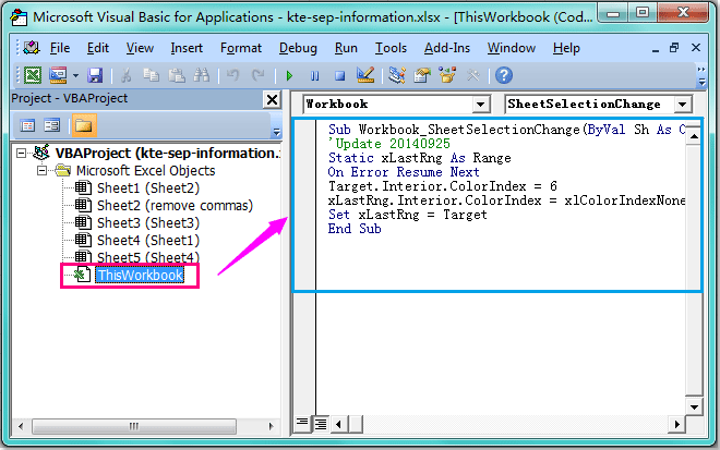
3。 次に、このコードを保存して閉じ、ワークシートに戻ります。セルまたは選択範囲を選択すると、選択したセルが強調表示され、選択したセルの変更に応じて動的に移動します。

注意:

1.見つからない場合 プロジェクトエクスプローラーペイン ウィンドウで、をクリックできます 詳しく見る > プロジェクトエクスプローラー セクションに Microsoft Visual Basic forApplicationsウィンドウ それを開く。

2.上記のコードでは、変更できます .ColorIndex = 6 あなたが好きな他の色への色。

3.このVBAコードは、ブック内のすべてのワークシートに適用できます。

4.ワークシートに色付きのセルがある場合、セルをクリックしてから他のセルに移動すると、色が失われます。


関連記事:

Excelでアクティブセルの行と列を自動ハイライトする方法は?

最高のオフィス生産性向上ツール

🤖 Kutools AI アシスタント: 以下に基づいてデータ分析に革命をもたらします。 インテリジェントな実行   |  コードを生成  |  カスタム数式の作成  |  データを分析してグラフを生成する  |  Kutools関数を呼び出す...
人気の機能: 重複を検索、強調表示、または識別する   |  空白行を削除する   |  データを失わずに列またはセルを結合する   |   数式なしのラウンド ...
スーパールックアップ: 複数の基準の VLookup    複数の値の VLookup  |   複数のシートにわたる VLookup   |   ファジールックアップ ....
詳細ドロップダウン リスト: ドロップダウンリストを素早く作成する   |  依存関係のドロップダウン リスト   |  複数選択のドロップダウンリスト ....
列マネージャー: 特定の数の列を追加する  |  列の移動  |  Toggle 非表示列の表示ステータス  |  範囲と列の比較 ...
注目の機能: グリッドフォーカス   |  デザインビュー   |   ビッグフォーミュラバー    ワークブックとシートマネージャー   |  リソースライブラリ (自動テキスト)   |  日付ピッカー   |  ワークシートを組み合わせる   |  セルの暗号化/復号化    リストごとにメールを送信する   |  スーパーフィルター   |   特殊フィルター (太字/斜体/取り消し線をフィルター...) ...
上位 15 のツールセット12 テキスト ツール (テキストを追加, 文字を削除する、...)   |   50+ チャート 種類 (ガントチャート、...)   |   40+ 実用的 (誕生日に基づいて年齢を計算する、...)   |   19 挿入 ツール (QRコードを挿入, パスから画像を挿入、...)   |   12 変換 ツール (数字から言葉へ, 通貨の換算、...)   |   7 マージ&スプリット ツール (高度な結合行, 分割セル、...)   |   ... もっと

Kutools for Excel で Excel スキルを強化し、これまでにない効率を体験してください。 Kutools for Excelは、生産性を向上させ、時間を節約するための300以上の高度な機能を提供します。  最も必要な機能を入手するにはここをクリックしてください...

説明


Officeタブは、タブ付きのインターフェイスをOfficeにもたらし、作​​業をはるかに簡単にします

  • Word、Excel、PowerPointでタブ付きの編集と読み取りを有効にする、パブリッシャー、アクセス、Visioおよびプロジェクト。
  • 新しいウィンドウではなく、同じウィンドウの新しいタブで複数のドキュメントを開いて作成します。
  • 生産性を 50% 向上させ、毎日何百回もマウス クリックを減らすことができます!
Comments (16)
No ratings yet. Be the first to rate!
This comment was minimized by the moderator on the site
I had the same problem, read the whole page and comments. While thinking to apply it or not, I was just randomly clicking on number and letters to select the whole column and rows. Then suddenly highlight of selected cell feature came back :)
This comment was minimized by the moderator on the site
Hello, if someone can help me... I pick up this code in internet (apologies to the owner). It does almost what i need but this code select the entirerow. What i need is a change that alow to select just the first two cells of the row of the activecells. When i click in the cell, i need that the cell of the column "$I16" and "$J16" (16 is the first line of my table) of that row became interior color (=9359529). The code is this: 
Dim lTarget As Range

Private Sub Worksheet_SelectionChange(ByVal Target As Range)

If Target.Row >= 16 Then

If Not lTarget Is Nothing Then

lTarget.EntireRow.Interior.ColorIndex = 0
End If

Target.EntireRow.Interior.Color = 9359529

Set lTarget = Target
End If
End Sub

Can you help me? I had try to change this code but the only thing i can as the select the interior color of the cell target and not the column "$I" and "$J" in that specific row.Thank you for your help.
Luis Lopes
This comment was minimized by the moderator on the site
I know that you proposed a solution but the solution comes with another problem as you described below: "The only problem with having this code active is that you can no longer change the active cell color as it changes back to what it was before you clicked it. I suggest that if you need to change the highlight colors on the sheet, do so with macros disabled or change the sub name for a second so it doesn't trigger when you are clicking on cells". This is not an acceptable alternative for me. I need to be able to change the colors in the cells when the macro is active. Do you have a solution for this this problem. If you come up with a solution for this problem please republish your corrected macro the new macro in full (rather than proposing patches to your original macro because I am technically challenged as far as macro are concerned).
This comment was minimized by the moderator on the site
I tried your macro by copying and pasting it into my Excel file. I did change one thing in the macro though. I changed the color index from 6 to 24 (to a color different than the colors I am currently using in my macro). It worked very nicely and I liked it a lot but then started causing a problem for me. I have a lot of cells filled with with colors in my Excel. The macro started removing the color fill from every cell touched. I don't know how to stop the macro's this odd behavior. I did not have any choice but to remove the macro from my file. I still like to use this macro if someone can help me to fix it.
This comment was minimized by the moderator on the site
That was super helpful, thank you.
This comment was minimized by the moderator on the site
Anyway you can do the left adjacent cell to highlight instead of active cell? Or a range of cells around the activecell?
This comment was minimized by the moderator on the site
Thank you, but use this with caution. It has the undesirable counter effect of not letting undo. Is there any solution for that?
This comment was minimized by the moderator on the site
But i am unable to do undo option and lose the previously assigned cell color also.
Please provide solution
This comment was minimized by the moderator on the site
Perfect solution as I always tend to loose the track of the highlighted cell during "Find and Select" operation. Thanks a lot.
This comment was minimized by the moderator on the site
Great!! But what if I don't want to lose the previously assigned cell color? That would be greater to know.
This comment was minimized by the moderator on the site
Use a conditional format on the cells you want to protect.
This comment was minimized by the moderator on the site
Instead of "ColorIndex" which has a limited set of 255 values (meaning any custom colors are lost), use "Color" instead. You'll need to store the old value in a new static long variable and also generate the highlight color you want with the RGB function. The only problem with having this code active is that you can no longer change the active cell color as it changes back to what it was before you clicked it. I suggest that if you need to change the highlight colors on the sheet, do so with macros disabled or change the sub name for a second so it doesn't trigger when you are clicking on cells, then just rename it back to normal to "re-activate" it. Here is my code:

Sub Workbook_SheetSelectionChange(ByVal Sh As Object, ByVal Target As Excel.Range)

Static xLastRng As Range
Static xLastRngColor As Long

On Error Resume Next

xLastRng.Interior.Color = xLastRngColor
xLastRngColor = Target.Interior.Color
Target.Interior.Color = RGB(255, 255, 0) 'compose whatever highlight color you want with RGB values, I am using yellow here
Set xLastRng = Target

End Sub
This comment was minimized by the moderator on the site
work.... great...
This comment was minimized by the moderator on the site
Yes, I would like to know this as well. How would you keep the previously selected cells highlight for tracking purposes?
This comment was minimized by the moderator on the site
See my comment above.
There are no comments posted here yet
Load More
Please leave your comments in English
Posting as Guest
×
Rate this post:
0   Characters
Suggested Locations