Excelで日付とUnixタイムスタンプを相互に変換する方法は?
Unixタイムスタンプ(エポック時間やPOSIX時間とも呼ばれる)は、コンピュータでの日付と時刻の表現に一般的に使用されます。このチュートリアルでは、Excelで日付をUnixタイムスタンプに変換したり、その逆を行うための明確な手順を提供し、これらの形式をスムーズに処理できるようにします。
 日付をタイムスタンプに変換
日付をタイムスタンプに変換するには、数式を使用できます。
空白のセルを選択し、例えばセルC2を選んで、次の数式を入力します =(C2-DATE(1970,1,1))*86400 そして、 Enter キーを押します。必要であれば、オートフィルハンドルをドラッグしてこの数式を範囲全体に適用できます。これで、日付の範囲がUnixタイムスタンプに変換されました。

2クリックで時間を10進数の時間、分、または秒に変換
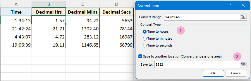
Kutools for Excelの「時間変換」機能は、時間を素早く10進数の時間、分、または秒に変換し、結果を元の場所または別の場所に配置するのに役立ちます。
日付と時刻をタイムスタンプに変換
日付と時刻をUnixタイムスタンプに変換するのに役立つ数式があります。
1. まず、協定世界時(UTC)をセルに入力します。例:1/1/1970。スクリーンショットをご覧ください:

2. 次に、この数式を入力します =(A1-$C$1)*86400 セルに入力し、 Enter キーを押します。必要であれば、オートフィルハンドルをドラッグしてこの数式を範囲全体に適用します。スクリーンショットをご覧ください:

ヒント: 数式において、A1は日付と時刻のセルを表し、C1は入力した協定世界時(UTC)です。
タイムスタンプを日付に変換
日付に変換するタイムスタンプのリストがある場合、以下の手順で行うことができます:
1. タイムスタンプのリストの隣にある空白のセルを選択し、この数式を入力します =(((A1/60)/60)/24)+DATE(1970,1,1), そして Enter キーを押します。その後、必要に応じてオートフィルハンドルをドラッグして必要な範囲に適用します。

2. 次に、数式を使用したセルを右クリックし、「セルの書式設定」を選択します。 Format Cells コンテキストメニューから選択し、表示される Format Cells ダイアログで、「Number 」タブをクリックし、「日付」を Date カテゴリ Category リストから選択し、右側のセクションで日付の形式を選択します。

3. 「OK」をクリックします。 OKすると、Unixタイムスタンプが日付に変換されているのが確認できます。

注意:
1. A1は変換したいタイムスタンプのセルを示します。
2. この数式は、タイムスタンプの系列を日付と時刻に変換するためにも使用でき、結果を日付と時刻の形式にフォーマットするだけです。
3. 上記の数式は10桁の数字を標準的な日時に変換しますが、11桁、13桁、または16桁の数字をExcelで標準的な日時に変換したい場合は、以下のような数式を使用してください:
11桁の数字を日付に変換: =A1/864000+DATE(1970,1,1)
13桁の数字を日付に変換: =A1/86400000+DATE(1970,1,1)
16桁の数字を日付に変換: =A1/86400000000+DATE(1970,1,1)
異なる長さの数字を日時に変換する場合、数式内の除数のゼロの数を調整して正しい結果を得ることができます。
関連記事:
Excelで異なるタイムゾーン間で日時を変換する方法は?
この記事では、Excelで異なるタイムゾーン間で日時を変換する方法を紹介します。
Excelでセル内の日付と時刻を2つの別々のセルに分割する方法は?
たとえば、日付と時刻が混在したデータのリストがあり、それぞれを2つのセルに分割したい場合、1つは日付、もう1つは時刻として表示したい場合があります。この記事では、Excelでこれを解決するための2つの簡単な方法を紹介します。
Excelで日付/時刻形式のセルを日付のみに変換する方法は?
日時形式のセルを日付値のみに変換したい場合(例:2016/4/7 1:01 AM → 2016/4/7)、この記事がお役に立てます。
Excelで日付から時刻を削除する方法は?
日付と時刻が含まれている列があり、時刻部分(例:12:23)を削除して、日付(例:2/17/2012)のみを残したい場合、Excelで複数のセルから時刻を迅速に削除する方法をご紹介します。
Excelで日付と時刻を1つのセルに結合する方法は?
ワークシートに2つの列があり、一方が日付、もう一方が時刻の場合、これら2つの列を1つに結合し、時刻形式を保持する方法が必要です。この記事では、Excelで日付列と時刻列を1つに結合し、時刻形式を保持する2つの方法を紹介します。
最高のオフィス業務効率化ツール
| 🤖 | Kutools AI Aide:データ分析を革新します。主な機能:Intelligent Execution|コード生成|カスタム数式の作成|データの分析とグラフの生成|Kutools Functionsの呼び出し…… |
| 人気の機能:重複の検索・ハイライト・重複をマーキング|空白行を削除|データを失わずに列またはセルを統合|丸める…… | |
| スーパーLOOKUP:複数条件でのVLookup|複数値でのVLookup|複数シートの検索|ファジーマッチ…… | |
| 高度なドロップダウンリスト:ドロップダウンリストを素早く作成|連動ドロップダウンリスト|複数選択ドロップダウンリスト…… | |
| 列マネージャー:指定した数の列を追加 |列の移動 |非表示列の表示/非表示の切替| 範囲&列の比較…… | |
| 注目の機能:グリッドフォーカス|デザインビュー|強化された数式バー|ワークブック&ワークシートの管理|オートテキスト ライブラリ|日付ピッカー|データの統合 |セルの暗号化/復号化|リストで電子メールを送信|スーパーフィルター|特殊フィルタ(太字/斜体/取り消し線などをフィルター)…… | |
| トップ15ツールセット:12 種類のテキストツール(テキストの追加、特定の文字を削除など)|50種類以上のグラフ(ガントチャートなど)|40種類以上の便利な数式(誕生日に基づいて年齢を計算するなど)|19 種類の挿入ツール(QRコードの挿入、パスから画像の挿入など)|12 種類の変換ツール(単語に変換する、通貨変換など)|7種の統合&分割ツール(高度な行のマージ、セルの分割など)|… その他多数 |
Kutools for ExcelでExcelスキルを強化し、これまでにない効率を体感しましょう。 Kutools for Excelは300以上の高度な機能で生産性向上と保存時間を実現します。最も必要な機能はこちらをクリック...
Office TabでOfficeにタブインターフェースを追加し、作業をもっと簡単に
- Word、Excel、PowerPointでタブによる編集・閲覧を実現。
- 新しいウィンドウを開かず、同じウィンドウの新しいタブで複数のドキュメントを開いたり作成できます。
- 生産性が50%向上し、毎日のマウスクリック数を何百回も削減!
全てのKutoolsアドインを一つのインストーラーで
Kutools for Officeスイートは、Excel、Word、Outlook、PowerPoint用アドインとOffice Tab Proをまとめて提供。Officeアプリを横断して働くチームに最適です。
- オールインワンスイート — Excel、Word、Outlook、PowerPoint用アドインとOffice Tab Proが含まれます
- 1つのインストーラー・1つのライセンス —— 数分でセットアップ完了(MSI対応)
- 一括管理でより効率的 —— Officeアプリ間で快適な生産性を発揮
- 30日間フル機能お試し —— 登録やクレジットカード不要
- コストパフォーマンス最適 —— 個別購入よりお得