Excelで今日よりも前の日付または後の日付に条件付き書式を適用するにはどうすればよいですか?
時間に敏感な情報の管理と追跡は、プロジェクト計画から請求書の期日や締め切りの監視まで、多くのExcelタスクにおいて重要です。頻繁に求められる要件の一つは、今日の日付よりも前または後の日付を目立たせることです。Excelの条件付き書式を使用すると、そのような日付を自動的に強調表示できるため、手動でデータをスクロールすることなく、期限切れのタスクや今後のイベントを迅速に見つけることができます。このチュートリアルでは、今日以前または以後の日付を強調表示するためのいくつかの実用的な方法を紹介します。組み込みのExcelツールとKutools for Excelを使用した拡張ソリューションの両方を取り上げます。大量のデータや更新頻度に関係なく、期日を効率的に強調したり、将来の活動をフラグ付けしたり、スプレッドシート全体の監視を維持する方法を学びます。
条件付き書式を使用して今日以前の日付や将来の日付を強調表示
次のスクリーンショットに示すように、いくつかの日付が含まれている列があるとします。すでに期日が過ぎている日付(今日より前)を強調表示したい場合や、計画や追跡を支援するために将来の日付を強調表示したい場合は、TODAY関数に基づいた数式を使用してExcelの条件付き書式を利用できます。この機能は、動的なデータを扱う際に特に価値があります。なぜなら、書式は毎日自動的に更新されるからです。

まず、日付のリストを選択します。この例では、セルA2:A15を選択します。ホームタブで「条件付き書式」>「ルールの管理」をクリックします。ガイダンスについては以下のスクリーンショットを参照してください:

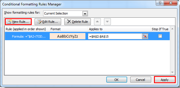
「条件付き書式ルール マネージャー」ダイアログが表示されたら、「新しいルール」ボタンをクリックしてカスタム数式ベースのルールを作成します。

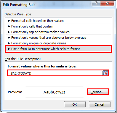
「新しい書式ルール」ダイアログでは:
• 「数式を使用して書式設定するセルを決定する」を選択します。このオプションにより、柔軟で日付駆動型のハイライトが可能です。
• 今日よりも前の日付を強調表示するには、次の数式を「この数式が真である場合の値を書式設定」フィールドにコピーして貼り付けます:
=$A2<TODAY()• 今日以降の日付(つまり今後の日付)を強調表示するには、次の数式を使用します:
=$A2>TODAY()• 次に、「書式」ボタンをクリックして希望の外観(塗りつぶしの色やフォントスタイルの変更など)を定義します。例を参照してください:
「セルの書式設定」ダイアログで希望の書式を指定します(例:期日や将来の日付を目立たせるために色を選択)、その後「OK」をクリックします。
「条件付き書式ルール マネージャー」に戻ると、新しく作成したルールが一覧に表示されています。ルールを有効にするには「適用」をクリックします。期日と未来の日付の両方を強調表示する場合は、他の数式を使用して2番目のルールを追加する手順を繰り返します。「ルール マネージャー」に戻ると、両方のルールが表示されます。
「OK」で確認すると、Excelシートは今日以前または以後の日付を目立たせ、アクションや注意を促す明確なインジケーターを提供します。期限切れの日付と今後の日付のフラグは、日々変わるにつれて自動的に更新され、常に最新かつ最も関連性のある項目を一目で確認できます。

結果は次の通りです:今日より前または後の日付が選択した形式で強調表示され、レビューとフォローアップが簡素化されました。

ヒントと注意点: 数式が正しく動作するように、日付セルが日付(テキストではない)としてフォーマットされていることを確認してください。予期しない結果が出る場合は、日付形式を再確認してください。非常に大きなデータセットの場合、条件付き書式がパフォーマンスに影響を与える可能性があるので、可能な限り書式範囲を制限することを検討してください。
Kutools AIを使用して今日以前の日付や将来の日付を強調表示
期限切れまたは将来の日付を簡単に強調表示するスマートな方法を探しているユーザーにとって、Kutools AI for Excelはプロセスを簡素化します。条件付き書式ルールを手動で構築する代わりに、平易な言葉でKutools AIに直接指示を出すことができます。この方法は、日付の強調表示を定期的に行う必要があるが、時間を節約したい場合や数式の設定を避けたい場合、また正確さと効率が重要な環境で作業する場合に理想的です。
今日との関係に基づいて日付を強調表示するためにKutools AIを使用するには:
- 「Kutools」>「AI アシスタント」をクリックして「KUTOOLS AI アシスタント」ペインを開き、次の操作を行います:
- 調べたい日付範囲を選択します。
- AI アシスタントペインに、次のようなコマンドを入力します:
— 期限切れの日付について: 選択した範囲で今日以前の日付を薄い青色で強調表示
— 将来の日付について: 選択した範囲で今日以降の日付を薄い青色で強調表示 - Enterキーを押すか「送信」をクリックします。Kutools AIはリクエストを分析します。処理が完了したら、「実行」をクリックして書式を自動的に適用します。
Kutools AIは意図を自動的に解釈し、適切な数式と書式を選択することで、時間を節約し、手動設定におけるエラーを最小限に抑えます。このアプローチは、動的なワークブック、数式に不慣れなユーザー、または大規模で頻繁に更新される日付リストを管理するユーザーにとって特に有用です。
注意: Kutools AIを使用するにはインターネット接続が必要であり、最新版のKutools for Excelがインストールされている必要があります。
Excelのヘルパー列数式を使用して日付をフラグ付けし分析する
多くの実世界のケースでは、単なるカラーコーディング以上のものが必要になることがあります。例えば、フィルタリング、ソート、または日付が今日以前または以後かどうかに基づいたレコードのカウントなどです。Excelの数式を使用したヘルパー列を使うことで、このようなケースを明確にフラグ立てでき、フィルタやピボットテーブルなどの他のExcel機能を使って詳細な分析を行うこともできます。
利点: 設定が簡単で、ソート/フィルタリングに対応し、特別な権限なしですべてのExcelバージョンで動作します。欠点: ヘルパー列のために追加のスペースが必要;条件付き書式と組み合わせない限り直接的な色付けは提供されません。
ヘルパー列を使った簡単な日付分析の方法は次のとおりです:
1. 日付リストの隣に新しい列を挿入します(例:A2:A15の日付の隣に列B)。
2. セルB2(A2が最初の日付であると仮定)に、次の数式を入力して期限切れの日付をフラグ付けします:
=A2<TODAY()この数式は、A2の日付が今日より前の場合にTRUEを返し、それ以外の場合はFALSEを返します。
3. あるいは、将来の日付を強調表示するには、次を使用します:
=A2>TODAY()4. 数式を確認するためにEnterキーを押してから、ハンドルをドラッグしてすべての日付を含む列を埋めます。TRUE/FALSEの結果は、期限切れまたは今後のステータスによってレコードをソートまたはフィルタリングするために使用できます。
明確なテキストラベルを好む場合、TRUE/FALSEをより記述的なフラグに置き換えてください。例:
=IF(A2<TODAY(),"Overdue",IF(A2>TODAY(),"Upcoming","Today"))必要なすべての行にこの数式をコピーします。フィルタリング、ソート、または条件付き書式やピボットテーブルなどの他のExcel機能で列を基準として使用できます。このアプローチは、レポート、ダッシュボード、または印刷可能な文書の準備に特に役立ちます。
注: 日付列が列Aではない場合、数式内の参照セルを適宜更新してください。整合性のない結果を避けるために、日付セルのデータタイプが日付(テキストではない)に設定されていることを確認してください。
関連記事:
- Excelで最初の文字/文字に基づいてセルに条件付き書式を適用するにはどうすればよいですか?
- Excelで#naを含むセルに条件付き書式を適用するにはどうすればよいですか?
- Excelで最初の出現を条件付き書式または強調表示するにはどうすればよいですか?
- Excelで負のパーセンテージを赤色で条件付き書式を適用するにはどうすればよいですか?
トラブルシューティングのヒント: 強調表示や数式が意図した通りに動作しない場合は、常に日付の書式と数式範囲を確認してください。条件付き書式の「プレビュー」機能を使用して、どのレコードが影響を受けているかを確認し、重複または矛盾するルールがないかを再確認してください。大きいテーブルの場合、ヘルパー列またはVBAマクロを使用するとメンテナンスが合理化され、頻繁な更新が必要な場合に時間を節約できます。最適なワークフローを見つけるために複数の方法を試してください。
最高のオフィス業務効率化ツール
| 🤖 | Kutools AI Aide:データ分析を革新します。主な機能:Intelligent Execution|コード生成|カスタム数式の作成|データの分析とグラフの生成|Kutools Functionsの呼び出し…… |
| 人気の機能:重複の検索・ハイライト・重複をマーキング|空白行を削除|データを失わずに列またはセルを統合|丸める…… | |
| スーパーLOOKUP:複数条件でのVLookup|複数値でのVLookup|複数シートの検索|ファジーマッチ…… | |
| 高度なドロップダウンリスト:ドロップダウンリストを素早く作成|連動ドロップダウンリスト|複数選択ドロップダウンリスト…… | |
| 列マネージャー:指定した数の列を追加 |列の移動 |非表示列の表示/非表示の切替| 範囲&列の比較…… | |
| 注目の機能:グリッドフォーカス|デザインビュー|強化された数式バー|ワークブック&ワークシートの管理|オートテキスト ライブラリ|日付ピッカー|データの統合 |セルの暗号化/復号化|リストで電子メールを送信|スーパーフィルター|特殊フィルタ(太字/斜体/取り消し線などをフィルター)…… | |
| トップ15ツールセット:12 種類のテキストツール(テキストの追加、特定の文字を削除など)|50種類以上のグラフ(ガントチャートなど)|40種類以上の便利な数式(誕生日に基づいて年齢を計算するなど)|19 種類の挿入ツール(QRコードの挿入、パスから画像の挿入など)|12 種類の変換ツール(単語に変換する、通貨変換など)|7種の統合&分割ツール(高度な行のマージ、セルの分割など)|… その他多数 |
Kutools for ExcelでExcelスキルを強化し、これまでにない効率を体感しましょう。 Kutools for Excelは300以上の高度な機能で生産性向上と保存時間を実現します。最も必要な機能はこちらをクリック...
Office TabでOfficeにタブインターフェースを追加し、作業をもっと簡単に
- Word、Excel、PowerPointでタブによる編集・閲覧を実現。
- 新しいウィンドウを開かず、同じウィンドウの新しいタブで複数のドキュメントを開いたり作成できます。
- 生産性が50%向上し、毎日のマウスクリック数を何百回も削減!
全てのKutoolsアドインを一つのインストーラーで
Kutools for Officeスイートは、Excel、Word、Outlook、PowerPoint用アドインとOffice Tab Proをまとめて提供。Officeアプリを横断して働くチームに最適です。
- オールインワンスイート — Excel、Word、Outlook、PowerPoint用アドインとOffice Tab Proが含まれます
- 1つのインストーラー・1つのライセンス —— 数分でセットアップ完了(MSI対応)
- 一括管理でより効率的 —— Officeアプリ間で快適な生産性を発揮
- 30日間フル機能お試し —— 登録やクレジットカード不要
- コストパフォーマンス最適 —— 個別購入よりお得