Excel でセルにテキスト、値、または空白が含まれている場合に行をハイライトするにはどうすればよいですか？

著者ケリー変更日2025-10-29

Excel で「Apple」の注文が見つかった行がハイライトされているスクリーンショット

Excel では、セルが特定のテキストや値を含んでいるか、あるいは空白かどうかといった条件に基づいて、該当する行を素早く見つけ出し、視覚的に強調表示することがよく求められます。条件に合致する行全体をハイライトすることで、可読性とデータ分析の効率が飛躍的に向上し、関連情報を一目で把握してスピーディーに対応できるようになります。

以下の方法は、さまざまなシナリオや要件に応じた実用的なソリューションを提供します。標準的なルールには条件付き書式を、インタラクティブな選択にはKutools for Excel の機能を、より動的または複雑な条件には高度な VBA コードをお選びいただけます。

条件付き書式を使用するを使用して、セルに特定のテキスト／値／空白が含まれる場合に行全体をハイライトする

Kutools for Excel を使用して、セルに特定のテキスト／値が含まれる場合に行全体をハイライトする

VBA コードを使用して、セルに特定のテキスト／値／空白が含まれる場合に行全体をハイライトする

別の列内の特定の値のいずれかをセルが含む場合に行全体をハイライトする

条件付き書式を使用するを使用して、セルに特定のテキスト／値／空白が含まれる場合に行をハイライトする

条件付き書式は、事前定義されたルールに基づいてセルや行の書式を自動的に適用するExcel の組み込み機能です。データが変更されるたびに書式を動的に更新したいシナリオに最適で、セルの値が特定の値と等しい、特定のテキストを含む、または空白であるといったシンプルな条件に特に適しています。

セルに特定のテキスト、特定の値、または空白が含まれている場合、テーブル内の該当する行全体をハイライトするには、次の手順に従ってください。

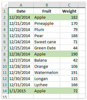
1。列見出しを除き、購入テーブルの関連する範囲（最初のデータ行から最後の行まで）のみを選択してください。ヘッダーセルの書式設定を避けるためです。

2。「ホーム」タブに移動し、「条件付き書式を使用する」＞「新しいルール」をクリックしてください。下記のスクリーンショットをご参照ください。
Excel の［新しい書式ルール］オプションのスクリーンショット

3。「新しい書式設定ルール」ダイアログボックスで、スクリーンショットのとおりにルールを設定します。
(1) 「ルールの種類の選択」で「数式を使用して書式設定するセルを決定」を選択します。
(2) 「次の数式を満たす値を書式設定」ボックスに、条件に一致する数式を入力します。

=$B2="Apple"

（3）「書式」ボタンをクリックしてください。
Excel の条件付き書式設定用［新しい書式ルール］ダイアログボックスのスクリーンショット

注記：

数式 =$B2="Apple"は、各行のセル B の値がテキスト「Apple」と完全に一致するかどうかをチェックします。$B2は、条件の基準となる実際の列に合わせて調整し、「Apple」は目的の値に変更してください。
セルが空白の行を強調表示するには、範囲を選択して=$B2=""を使用してください。
セルが特定のテキストで始まる行をハイライトしたい場合は、=LEFT($B2,5)="Apple"を使用できます。同様に、そのテキストで終わるセルを対象にするには、=RIGHT($B2,5)="Apple"を使いましょう。
条件付き書式で使用する数式は、デフォルトで大文字と小文字を区別しません。大文字と小文字を区別して一致させたい場合は、=EXACT($B2,"Apple")を使用してください。

4。「セルの書式設定」ダイアログボックスで「塗りつぶし」タブに切り替え、お好みのハイライト色を選んで「OK」をクリックします。
Excel で背景色が選択されている［セルの書式設定］ダイアログボックスのスクリーンショット

5。「OK」を再度クリックして、「新しい書式設定ルール」ダイアログボックスを閉じましょう。

これらの手順を完了すると、指定した条件に一致する範囲内のすべての行が自動的にハイライトされます。後で値を編集しても、ハイライトは自動的に更新されます。

実用的なヒント：条件付き書式では、複数のルールを同時に使用できます。さまざまな条件に基づいて、異なる色で行の範囲を重ねて強調表示することが可能です。ルールが正しく機能しないように見える場合は、適用範囲の選択と数式内の参照スタイルを今一度ご確認ください。書式設定を削除するには、「条件付き書式」メニュー内の「ルールのクリア」をご利用ください。

メリット：動的でセルの変更に自動追随し、アドイン不要。
デメリット：非常に複雑または多面的な条件には不向きで、大規模ファイルでは動作が遅くなる可能性があります。

Kutools for Excel を使用して、セルに特定のテキスト／値が含まれる場合に行をハイライトする

Kutools for Excel は、テーブル内のデータ選択と書式設定をより簡単かつ効率的に行えるユーザーフレンドリーな機能を提供します。「特定のセルを選択する」機能を使えば、特定のテキストや値を含むセルに基づいて素早く行を選択し、手動でハイライト色を適用できます。

Kutools for Excelは300 以上の高度な機能を提供し、複雑な作業を効率化して、創造性と生産性を高めます。AI 機能と統合されたKutools は、正確にタスクを自動化し、データ管理を簡単にします。Kutools for Excel の詳細情報。。。 無料トライアル。。。

1。特定のテキストまたは値を検索する列を選択してください。最初の関連セルから始めて、チェックしたいすべてのエントリが含まれるようにしてください。

2。「Kutools」＞「選択」＞「特定のセルを選択」をクリックします。
Kutools for Excel「特定のセルを選択」機能のダイアログボックスのスクリーンショット

3。「特定のセルを選択する」ダイアログボックス（上記スクリーンショット参照）で、次の手順に従って操作してください。
(1) 「選択タイプ」の下にある「行全体」をチェックします。
(2) 「指定タイプ」のドロップダウンから「含む」を選択し、対象のテキストを入力します。
(3) 「OK」をクリックします。

4。フォローアップダイアログで「OK」をクリックして確定すると、関連するすべての行が自動的に選択されます。
成功ダイアログのスクリーンショット Kutools for Excel「特定のセルを選択」機能を適用した後にハイライトされた行を示すスクリーンショット

5。「ホーム」タブに戻り、「塗りつぶし色」をクリックしてドロップダウンからハイライトの色を選び、選択した行に書式を適用します。

Kutools を使えば、数式を入力したり複雑なメニューを操作したりする必要なく、データを素早く識別してカラーコードで表示できます。この方法は、継続的なルールに基づくハイライトではなく、特定の行を一度だけ選択・書式設定したい場合に特に効果的です。

実用的なヒント：Kutools を使用した後は、Excel の並べ替えやフィルター機能を使って、強調表示された行の範囲のみを操作できます。既存の書式設定が上書きされてしまう可能性があるため、塗りつぶし色を適用する前に、選択された行を必ず確認してください。

メリット：操作が素早く、インタラクティブで、数式は不要。幅広い条件を組み込みロジックで処理できます。
デメリット：動的ではないため、新規データが追加された際には再度プロセスを実行する必要があります。また、Kutools for Excel のインストールが必須です。

Kutools for Excel— 300 以上の必須ツールでExcel を強化し、作業をより迅速・簡単に。AI 機能を活用して、スマートなデータ処理と生産性の飛躍的な向上を実現します。今すぐ入手

VBA コードを使用して、セルに特定のテキスト／値／空白が含まれる場合に行全体をハイライトする

条件付き書式の機能やKutools の範囲を超えて、より高度で動的な条件に基づいて行をハイライトしたいユーザーにとって、VBA（Visual Basic for Applications）は強力な自動化手段を提供します。この方法は、リスト内の任意の値を含む行、複数の列にわたる条件を満たす行、複雑なパターンに一致する行など、さまざまなルールに基づいて対象範囲を絞り込み、コード実行時に即座に書式設定を適用したい場合に特に有効です。

準備：VBA を実行する前に、必ずワークブックを保存し、対象となる列と行の範囲を確認しておきましょう。VBA による変更は即座に適用されるため、バックアップがなければ元に戻すのが難しくなる場合があります。

1。VBA エディターを開くには、開発者ツール > Visual Basicをクリックしてください。表示されたMicrosoft Visual Basic for Applicationsウィンドウで、挿入 > 標準モジュールをクリックし、以下のコードをモジュールにコピー＆ペーストしてください：

Sub HighlightRowsByCellContent()
    Dim ws As Worksheet
    Dim rng As Range
    Dim lastRow As Long
    Dim targetCol As String
    Dim searchValue As String
    Dim cell As Range
    Dim xTitleId As String
    Dim i As Long
    
    On Error Resume Next
    Set ws = Application.ActiveSheet
    xTitleId = "KutoolsforExcel"
    
    ' Prompt for the target column by letter (e.g., "B") and the value to search for
    targetCol = Application.InputBox("Enter the column letter to check (e.g., B):", xTitleId, "B", Type:=2)
    searchValue = Application.InputBox("Enter the text/value to search for (leave blank to find blank cells):", xTitleId, "", Type:=2)
    
    lastRow = ws.Cells(ws.Rows.Count, targetCol).End(xlUp).Row
    
    ' Loop through each row and highlight if criteria match
    For i = 2 To lastRow
        Set cell = ws.Cells(i, Columns(targetCol).Column)
        If searchValue = "" Then
            If Trim(cell.Value) = "" Then
                ws.Rows(i).Interior.Color = vbYellow
            End If
        Else
            If InStr(1, cell.Value, searchValue, vbTextCompare) > 0 Then
                ws.Rows(i).Interior.Color = vbYellow
            End If
        End If
    Next i
End Sub

2。コードを実行するには、VBA ウィンドウの（実行ボタン）をクリックしてください。プロンプトが表示されるので、対象列と値を指定します（空白セルに一致させる場合は、値を空欄のままにしてください）。アクティブなワークシート内で条件に該当するすべての行が、黄色でハイライトされます！

パラメーターの説明および詳細オプション：

targetCol：チェック対象の列をアルファベットで指定してください（例：「B」を入力すると、各行の B 列がチェックされます）。
searchValue：検索したいテキストまたは値を入力してください。空白セルを検索する場合は、このボックスを空欄のままにしておけば OK です。
Interior.Color：コードではハイライト色として黄色（)vbYellow）を使用しています。これをvbGreenやvbCyanに変更するか、RGB(r,g,b)を使ってカスタムカラーを指定することもできます！

ヒントと注意事項：

マクロを実行する前に、必ずワークブックを保存してください。書式設定は即座に適用されます。
後でハイライトをクリアしたい場合は、ws.Rows(i).Interior.ColorIndex = xlNone を実行する類似のマクロを設定してください。
この VBA はアクティブなワークシート上で動作します。他のシートで使う場合は、Set ws = Worksheets("SheetName")の部分を調整してください。
大規模なデータセットの処理には、数秒かかる場合があります。

トラブルシューティング：コードが強調表示された行の範囲しない場合は、以下の原因を確認してください：

列はアルファベットで指定してください。列番号ではなく、常にアルファベットを入力するようにしてください。
行数の設定は、データテーブルの先頭（例：ヘッダーが行1 にある場合、行2 から開始）から始まる必要があります。

メリット：柔軟性が非常に高く、複雑な条件にも対応可能。高度なシナリオに合わせてカスタマイズできます。
デメリット：VBA に関するある程度の知識が必要で、手動で設定した書式が上書きされる可能性があります。

別の列にある特定の値のいずれかをセルが含む場合に行全体をハイライト

セルの値が別の列にあるリスト内のいずれかの値と一致する場合にのみ、その行を強調表示したいケースがあります。たとえば、商品名の列があり、指定リスト内のいずれかの商品名と一致するすべての行を自動的にハイライトしたい場合などが該当します。Kutools for Excel の「範囲比較」ユーティリティを使えば、複雑な数式を使わずにこれを簡単に実現できます。

1。「Kutools」＞「選択」＞「同じ／異なるセルを選択」を順にクリックします。
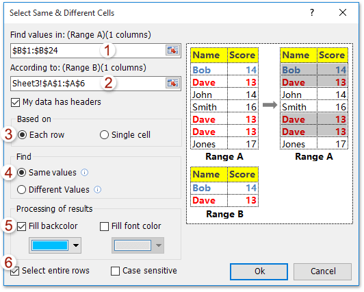
Excel の Kutools タブにある Kutools for Excel「同じセルと異なるセルを選択」オプションのスクリーンショット

2。「同じ/異なるセルを選択」ダイアログボックスで、次のように設定してください。

「値を検索する範囲」で、一致を確認したい列を指定してください。
「基準」で、特定の値のリストを含む列を選択してください。
「基準」の下にある「各行」にチェックを入れます。
「検索」の下にある「同じ値」を選択してください。
「選択結果の処理」の下にある「背景色を塗りつぶす」を有効にして、お好みの色を選択してください。
「行全体を選択」にチェックが入っていることをご確認ください。

Kutools for Excel「同じセルと異なるセルを選択」ダイアログボックスのスクリーンショット

3。「OK」をクリックしてユーティリティを実行すると、マッチした行数とハイライト結果が通知されます。「OK」をクリックすると、ダイアログが閉じます。
成功ダイアログのスクリーンショット

その結果、指定したセルの値が参照列のいずれかの値と一致する行が強調表示された範囲が表示されます。
Kutools for Excel を使用して別の列の値に基づいて行をハイライトした結果を示すスクリーンショット

この手法は、リスト間でデータを照合する際に特に役立ちます（例：商品コードを有効在庫リストと照合したり、顧客グループに関連するすべての取引を特定したりする場合など）。

ヒント：値リストが大きい場合は、比較を実行する前にExcel の「重複を削除」機能でデータをクリーンアップしましょう。両方の列に余分なスペースや結果に影響を与えるような差異がないか、必ず確認してください。データを変更しても書式は自動更新されないため、再度処理を実行する必要があります。

メリット：リスト間の照合に最適で、行をまとめて選択・ハイライトできます。
デメリット：Kutools アドインが必要で、自動では動作しないため、データを変更するたびに再実行が必要です。

デモ：セルがある特定の値または指定値のいずれかを含む場合に行をハイライト

Kutools for Excel：300 個を超える便利なツールがすぐそこへ！AI 搭載の機能で、よりスマートでスピーディーな作業をぜひお楽しみください！今すぐダウンロード！

Excel で特定のセルが空白の場合は保存を防止するには、どうすればよいですか？

Excel でセルが空白の場合に計算（数式）を無視する方法は？

Excel で IF 関数に AND、OR、NOT を組み合わせるにはどうすればよいですか？

Excel でセルが空白のときに警告やアラートメッセージを表示するには、どうすればよいですか？

Excel でセルが空白の場合に表示するテキストやメッセージを入力するには、どうすればよいですか？

Excel で長いリスト内のセルが空白の場合、その行を削除するにはどうすればよいですか？

最高の Office 業務効率化ツール

🤖	KUTOOLS AI アシスタント：次に基づいてデータ分析を革新します：インテリジェント実行｜コード生成｜カスタム数式作成｜データ分析とチャート生成｜拡張機能呼び出し…
	人気の機能：検索・ハイライト、または重複をマーキング｜空白行を削除する｜データを失うことなく列の結合またはセルを｜数式を使用しない四捨五入...
	スーパー LOOKUP：複数条件 VLookup ｜複数値 VLookup ｜複数シート間 VLookup ｜ファジーマッチ....
	高度なドロップダウンリスト：ドロップダウンリストをすばやく作成｜連動型ドロップダウンリスト｜複数選択可能なドロップダウンリスト....
	列マネージャー：指定した数の列を追加｜列の移動｜非表示列の表示状態を切り替え｜範囲および列の比較...
	注目の機能：グリッドフォーカス｜デザインビュー｜強化された数式バー｜ワークブックとシートマネージャー｜リソースライブラリ（オートテキスト）｜日付ピッカー｜ワークシートの統合｜暗号化／セルの復号化｜リストからメール送信｜スーパーフィルター｜特殊フィルタ（太字のフォントを持つセルをフィルタリング／斜体／取り消し線。。。）。。。
	トップ15 ツールセット：12 テキストツール（テキストの追加、特定の文字を削除、...）｜ 50+チャートタイプ（ガントチャート、...）｜ 40+実用的関数（誕生日に基づいて年齢を計算します、...）｜ 19 挿入ツール（QR コードを挿入、パスから画像を挿入、...）｜ 12 変換ツール（単語に変換する、為替レートの変換、...）｜ 7 結合と分割ツール（高度な行のマージ、セルの分割、...）｜さらに多数

Kutools はお好みの言語でご利用いただけます。英語、スペイン語、ドイツ語、フランス語、中国語、および40+の他の言語をサポートしています！

Kutools for Excel でExcel スキルを強化し、これまでにない効率を体験しましょう。Kutools for Excel は、生産性を高め、時間を大幅に節約できる高度な機能を300 以上提供します。最も必要な機能を今すぐ入手するにはこちらをクリック。。。

Kutools for Excel の詳細はこちら。。。無料ダウンロード。。。

Office Tab は Office にタブインターフェースをもたらし、作業を大幅に簡単にします

Word、Excel、PowerPoint でタブを使った編集と閲覧を有効にします。Publisher、Access、Visio、Project でもご利用いただけます。
複数のドキュメントを、新しいウィンドウではなく、同じウィンドウ内の新しいタブで開いたり作成したりできます。
日々の生産性を50％も向上させ、毎日数百回ものマウスクリックを削減します！