ExcelでVLOOKUPを使用して、複数の対応する値を水平方向に返す方法は？

Author Sun Last modified 2025-08-26

デフォルトでは、VLOOKUP関数はExcelで垂直レベルに対応する複数の値を返すことができます。しかし、場合によっては、以下のように水平レベルで複数の値を返したい場合があります。ここで、このタスクを解決できる数式をご紹介します。
VLOOKUPで複数の値を水平方向に返す

VLOOKUPで複数の値を水平方向に返す

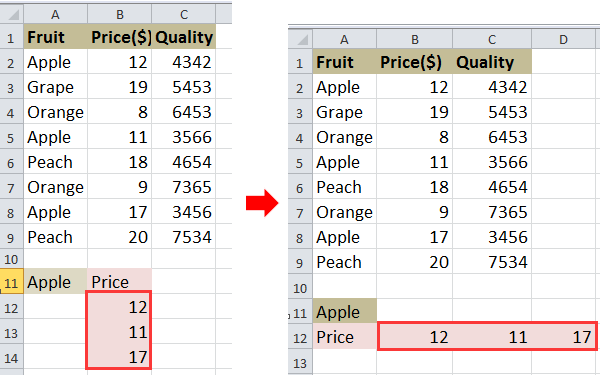
例えば、以下のスクリーンショットのようなデータ範囲があり、リンゴの価格をVLOOKUPで検索したいとします。
sample data

1. セルを選択し、この数式を入力します =INDEX($B$2:$B$9, SMALL(IF($A$11=$A$2:$A$9, ROW($A$2:$A$9)-ROW($A$2)+1), COLUMN(A1))) それを入力し、次に押します Shift + Ctrl + Enter そして、オートフィルハンドルを右にドラッグして、この数式を適用します。 #NUM! が表示されるまで続けます。スクリーンショットをご覧ください：
VLOOKUP and return multiple values horizontally with formula

2. 次に、#NUM! を削除します。スクリーンショットをご覧ください：
delete the error cells

ヒント: 上記の数式では、B2:B9は返したい値がある列範囲、A2:A9は検索値が含まれる列範囲、A11は検索値、A1はデータ範囲の最初のセル、A2は検索値が含まれる列範囲の最初のセルです。

複数の値を垂直方向に返したい場合は、こちらの記事「Excelで検索値に基づいて複数の対応する値を返す方法」を参照してください。

Kutools AIでExcelの魔法を解き放つ

スマート実行: セル操作、データ分析、グラフ作成を簡単なコマンドで行います。
カスタム数式: ワークフローを合理化するための独自の数式を生成します。
VBAコーディング: 簡単にVBAコードを作成し実装します。
数式の解釈: 複雑な数式を簡単に理解できます。
テキスト翻訳: スプレッドシート内の言語障壁を取り除きます。

AI搭載ツールでExcelの機能を強化しましょう。今すぐダウンロードして、かつてないほどの効率を体験してください！

最高のオフィス業務効率化ツール

🤖	Kutools AI Aide：データ分析を革新します。主な機能：Intelligent Execution｜コード生成｜カスタム数式の作成｜データの分析とグラフの生成｜Kutools Functionsの呼び出し……
	人気の機能：重複の検索・ハイライト・重複をマーキング｜空白行を削除｜データを失わずに列またはセルを統合｜丸める……
	スーパーLOOKUP：複数条件でのVLookup｜複数値でのVLookup｜複数シートの検索｜ファジーマッチ……
	高度なドロップダウンリスト：ドロップダウンリストを素早く作成｜連動ドロップダウンリスト｜複数選択ドロップダウンリスト……
	列マネージャー：指定した数の列を追加｜列の移動｜非表示列の表示/非表示の切替｜範囲＆列の比較……
	注目の機能：グリッドフォーカス｜デザインビュー｜強化された数式バー｜ワークブック＆ワークシートの管理｜オートテキストライブラリ｜日付ピッカー｜データの統合｜セルの暗号化/復号化｜リストで電子メールを送信｜スーパーフィルター｜特殊フィルタ（太字/斜体/取り消し線などをフィルター）……
	トップ15ツールセット：12 種類のテキストツール（テキストの追加、特定の文字を削除など）｜50種類以上のグラフ（ガントチャートなど）｜40種類以上の便利な数式（誕生日に基づいて年齢を計算するなど）｜19 種類の挿入ツール（QRコードの挿入、パスから画像の挿入など）｜12 種類の変換ツール（単語に変換する、通貨変換など）｜7種の統合＆分割ツール（高度な行のマージ、セルの分割など）｜… その他多数