Excel で毎月の最初または最後の金曜日をどのように見つけますか?
通常、金曜日はその月の最終営業日です。Excel で指定された日付に基づき、その月の最初または最後の金曜日を簡単に見つけるにはどうすればよいでしょうか?本記事では、毎月の最初または最後の金曜日を正確に求められる2 つの数式の使い方を詳しくご紹介します。
月の最初の金曜日を見つける
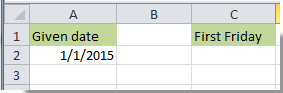
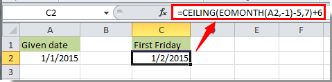
たとえば、下図のようにセル A2 に日付「2015/1/1」が入力されている場合、この日付に基づいて当該月の最初の金曜日を求めるには、以下の手順を実行してください。
1。結果を表示するセル(ここではセル C2)を選択します。
2。以下の数式をコピーして貼り付け、Enter キーを押してください。
=CEILING(EOMONTH(A2,-1)-5,7)+6
注記:
月の最後の金曜日を見つける
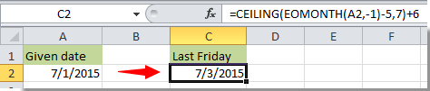
セル A2 に日付「2015/1/1」が入力されている場合、Excel でこの月の最後の金曜日を求めるには、以下の手順を実行してください。
1。セルを選択して、次の数式をコピー&ペーストし、Enter キーを押して結果を表示しましょう。
=DATE(YEAR(A2),MONTH(A2)+1,0)+MOD(-WEEKDAY(DATE(YEAR(A2),MONTH(A2)+1,0),2)-2,-7)

注記:数式内の A2 は、指定された日付が入力されている参照セルです。必要に応じて変更してください。
関連記事:
- Excel でリスト内の最小値と最大値を5 つずつ見つけるには、どうすればよいでしょうか?
- Excel で特定のブックが開いているかどうかを確認するには、どうすればよいでしょうか?
- Excel でセルが他のセルから参照されているかどうかを確認するには、どうすればよいでしょうか?
- Excel でリストの中から今日に最も近い日付をどうやって見つけますか?
最高の Office 業務効率化ツール
| 🤖 | KUTOOLS AI アシスタント:次に基づいてデータ分析を革新します:インテリジェント実行 | コード生成| カスタム数式作成 | データ分析とチャート生成| 拡張機能呼び出し… |
| 人気の機能:検索・ハイライト、または重複をマーキング | 空白行を削除する | データを失うことなく列の結合またはセルを | 数式を使用しない四捨五入... | |
| スーパー LOOKUP:複数条件 VLookup | 複数値 VLookup | 複数シート間 VLookup | ファジーマッチ.... | |
| 高度なドロップダウンリスト:ドロップダウンリストをすばやく作成 | 連動型ドロップダウンリスト | 複数選択可能なドロップダウンリスト.... | |
| 列マネージャー:指定した数の列を追加|列の移動|非表示列の表示状態を切り替え|範囲および列の比較... | |
| 注目の機能:グリッドフォーカス | デザインビュー |強化された数式バー | ワークブックとシートマネージャー | リソースライブラリ(オートテキスト)| 日付ピッカー | ワークシートの統合 | 暗号化/セルの復号化 | リストからメール送信 | スーパーフィルター | 特殊フィルタ(太字のフォントを持つセルをフィルタリング/斜体/取り消し線。。。) 。。。 | |
| トップ15 ツールセット:12 テキストツール(テキストの追加、特定の文字を削除、...)| 50+チャートタイプ(ガントチャート、...)| 40+実用的関数(誕生日に基づいて年齢を計算します、...)| 19 挿入ツール(QR コードを挿入、パスから画像を挿入、...)| 12 変換ツール(単語に変換する、為替レートの変換、...)| 7 結合と分割ツール(高度な行のマージ、セルの分割、...)|さらに多数 |
Kutools for Excel でExcel スキルを強化し、これまでにない効率を体験しましょう。Kutools for Excel は、生産性を高め、時間を大幅に節約できる高度な機能を300 以上提供します。最も必要な機能を今すぐ入手するにはこちらをクリック。。。
Office Tab は Office にタブインターフェースをもたらし、作業を大幅に簡単にします
- Word、Excel、PowerPoint でタブを使った編集と閲覧を有効にします。Publisher、Access、Visio、Project でもご利用いただけます。
- 複数のドキュメントを、新しいウィンドウではなく、同じウィンドウ内の新しいタブで開いたり作成したりできます。
- 日々の生産性を50%も向上させ、毎日数百回ものマウスクリックを削減します!
すべてのKutools アドインが、たった1 つのインストーラーで完結。
Kutools for Officeスイートには、Excel ・Word ・Outlook ・PowerPoint 用のアドインと Office Tab Pro が含まれており、複数の Office アプリを横断して作業するチームに最適です。
- オールインワンスイート— Excel、Word、Outlook、PowerPoint 用アドイン+Office Tab Pro
- インストーラー1 つ、ライセンス1 つ— 数分でセットアップ可能(MSI 対応)
- 連携してさらにパワーアップ— Office アプリ全体で生産性が向上
- 30 日間のフル機能トライアル— 登録不要、クレジットカード不要
- 最高のお得感— 個別アドイン購入よりお得