Excel で数式内の小数点以下の桁数を制限するにはどうすればよいですか?
たとえば、ある範囲を合計した結果、Excel で小数点以下4 桁の合計値が得られたとします。この合計値を、セルの書式設定ダイアログボックスを使って小数点以下1 桁に表示しようと考えるかもしれません。実は、数式内で直接小数点以下の桁数を制限することも可能です。本記事では、Excel でセルの書式設定コマンドを使用して小数点以下の桁数を制限する方法と、ROUND 関数を使って小数点以下の桁数を制限する方法をご紹介します。
- Excel で[セルの書式設定]コマンドを使用して小数点以下の桁数の桁数を制限する
- Excel で数式内の小数点以下の桁数の桁数を制限する
- 複数の数式内の小数点以下の桁数の桁数を一括で制限する
- 複数の数式内の小数点以下の桁数の桁数を制限する
Excel で[セルの書式設定]コマンドを使用して小数点以下の桁数の桁数を制限する
通常、Excel ではセルの書式設定を使って、小数点以下の桁数を簡単に制限できます。
1。小数点以下の桁数を制限したいセルを選択します。
2。選択したセルを右クリックし、コンテキストメニューからセルの書式設定を選択してください。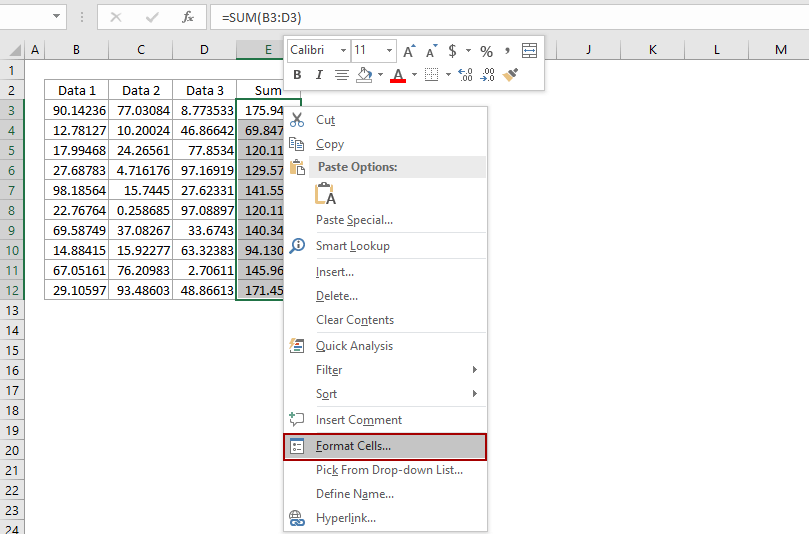
3。表示されるセルの書式設定ダイアログボックスで、数値タブに移動し、数値を分類ボックス内でクリックして選択し、続いて小数点以下の桁数ボックスに希望の数字を入力します。
たとえば、選択したセルの小数点以下の桁数を1 桁に制限したい場合は、1を小数点以下の桁数ボックスに入力してください。下記のスクリーンショットをご確認ください: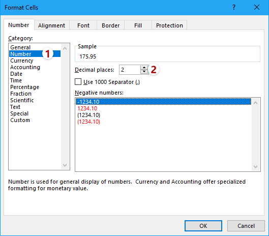
4。セルの書式設定ダイアログボックスでOKをクリックすると、選択したセルの小数点以下の桁数がすべて指定した小数位数に変更されます。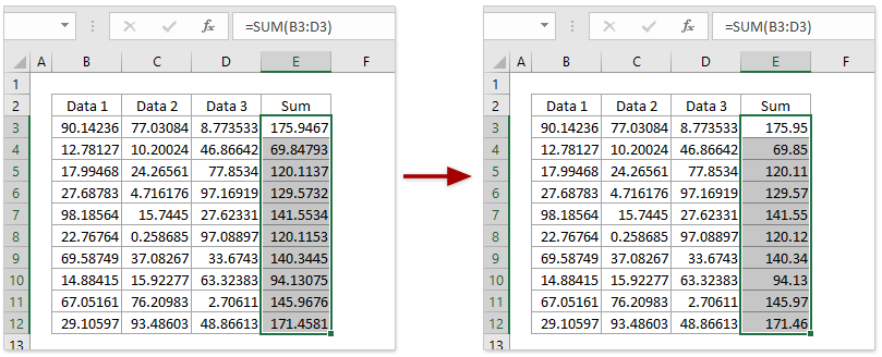
注:セルを選択した後、リボンのホームタブにある数値グループ内の小数点表示桁上げボタン![]() または小数点表示桁下げボタン
または小数点表示桁下げボタン![]() を直接クリックして、小数点以下の桁数を変更できます。
を直接クリックして、小数点以下の桁数を変更できます。
Excel で複数の数式内の小数点以下の桁数の桁数を簡単に制限する
一般的に、=ROUND(元の数式, 桁数)を使えば、1 つの数式内で小数点以下の桁数を簡単に制限できます。しかし、複数の数式を1 つずつ手動で修正するのは非常に面倒で時間がかかります。そんなときは、Kutools for Excel の[操作]機能を使えば、複数の数式内の小数点以下の桁数を一括で簡単に制限できます!
Kutools for Excel— 300 以上の必須ツールでExcel を強化し、作業をより迅速・簡単に。AI 機能を活用して、スマートなデータ処理と生産性の飛躍的な向上を実現します。今すぐ入手
Excel で数式内の小数点以下の桁数の桁数を制限する
たとえば、一連の数値の合計を計算していて、その合計値の数式内で小数点以下の桁数を制限したい場合は、Excel でどのように実現できるでしょうか?そのような場合には、ROUND 関数をお試しください。
基本的な ROUND 関数の構文は次のとおりです:
=ROUND(数値、 桁数)
他の数式と ROUND 関数を組み合わせる場合は、次のように構文を変更してください。
=ROUND(元の数式、 桁数)
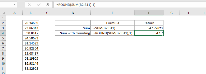
今回のケースでは、合計値の小数点以下を1 桁に制限したいので、次の数式を適用できます。
=ROUND(SUM(B2:B11),1)
複数の数式内の小数点以下の桁数の桁数を一括で制限する
お使いの環境にKutools for Excelがインストール済みの場合、その操作機能を使えば、Excel 上の複数の既存数式を一括で簡単に修正(たとえば四捨五入の設定など)できます。以下の手順に従ってください:
Kutools for Excel— Excel 用の便利なツールを300 種類以上搭載!全機能が30 日間、クレジットカード不要で無料でお試しいただけます。今すぐ入手
1。小数点以下の桁数を制限したい数式セルを選択し、Kutools>その他>操作をクリックします。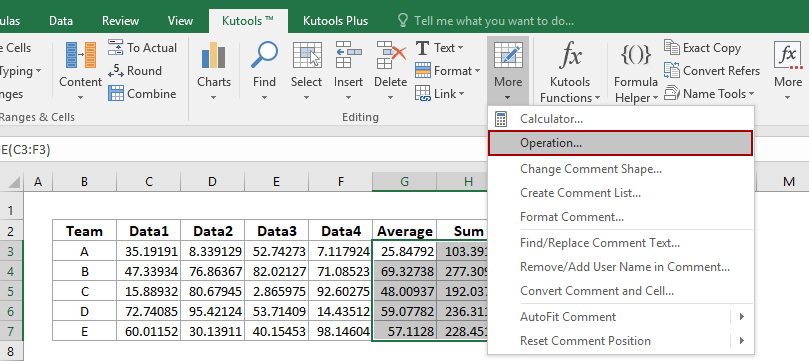
2。計算ツールダイアログで、四捨五入を操作リストボックスから選択し、オペランドセクションに小数点以下の桁数を入力して、数式を作成オプションをオンにします。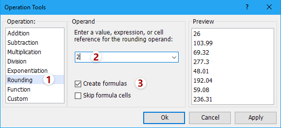
3。OKボタンをクリックします。
これで、すべての数式セルが指定された小数点以下の桁数に一括で四捨五入されたことをご確認いただけます。スクリーンショットをご覧ください:
ヒント:複数の数式セルを一括で切り捨てまたは切り上げたい場合は、次のように設定してください。計算ツールダイアログで、(1)[操作]リストボックスからカスタムを選択し、(2)[カスタム]セクションに=ROUNDUP(?, 2)または=ROUNDDOWN(?, 2)を入力してから、(3)数式を作成オプションをオンにします。スクリーンショットをご覧ください: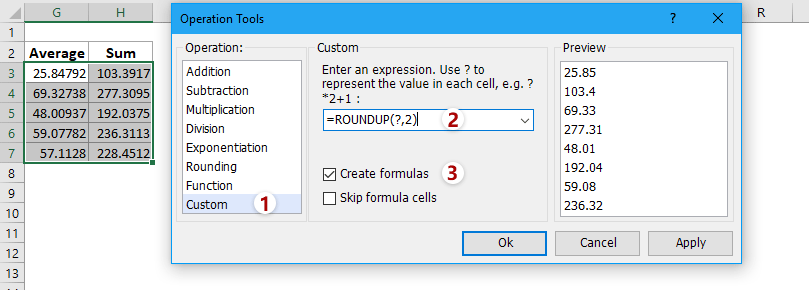
Excel で複数の数式内の小数点以下の桁数の桁数を簡単に制限する
通常、「小数点表示桁下げ」機能を使うと、セル内の小数点以下の表示桁数を減らせますが、数式バーに表示される実際の値はまったく変わりません。Kutools for Excelの四捨五入ユーティリティを使えば、指定した小数点以下の桁数に応じて、値を切り上げ・切り捨て・偶数丸めできます。
Kutools for Excel—Excel 用の便利なツールを300 以上搭載!全機能をクレジットカード不要で60 日間無料でお試しいただけます。今すぐ入手
この方法により、数式セルが指定された小数点以下の桁数の桁数に一括で四捨五入されますが、これらのセルから数式が削除され、四捨五入後の結果のみが残ります。
デモ:Excel で数式内の小数点以下の桁数の桁数を制限する
関連記事:
最高の Office 業務効率化ツール
| 🤖 | KUTOOLS AI アシスタント:次に基づいてデータ分析を革新します:インテリジェント実行 | コード生成| カスタム数式作成 | データ分析とチャート生成| 拡張機能呼び出し… |
| 人気の機能:検索・ハイライト、または重複をマーキング | 空白行を削除する | データを失うことなく列の結合またはセルを | 数式を使用しない四捨五入... | |
| スーパー LOOKUP:複数条件 VLookup | 複数値 VLookup | 複数シート間 VLookup | ファジーマッチ.... | |
| 高度なドロップダウンリスト:ドロップダウンリストをすばやく作成 | 連動型ドロップダウンリスト | 複数選択可能なドロップダウンリスト.... | |
| 列マネージャー:指定した数の列を追加|列の移動|非表示列の表示状態を切り替え|範囲および列の比較... | |
| 注目の機能:グリッドフォーカス | デザインビュー |強化された数式バー | ワークブックとシートマネージャー | リソースライブラリ(オートテキスト)| 日付ピッカー | ワークシートの統合 | 暗号化/セルの復号化 | リストからメール送信 | スーパーフィルター | 特殊フィルタ(太字のフォントを持つセルをフィルタリング/斜体/取り消し線。。。) 。。。 | |
| トップ15 ツールセット:12 テキストツール(テキストの追加、特定の文字を削除、...)| 50+チャートタイプ(ガントチャート、...)| 40+実用的関数(誕生日に基づいて年齢を計算します、...)| 19 挿入ツール(QR コードを挿入、パスから画像を挿入、...)| 12 変換ツール(単語に変換する、為替レートの変換、...)| 7 結合と分割ツール(高度な行のマージ、セルの分割、...)|さらに多数 |
Kutools for Excel でExcel スキルを強化し、これまでにない効率を体験しましょう。Kutools for Excel は、生産性を高め、時間を大幅に節約できる高度な機能を300 以上提供します。最も必要な機能を今すぐ入手するにはこちらをクリック。。。
Office Tab は Office にタブインターフェースをもたらし、作業を大幅に簡単にします
- Word、Excel、PowerPoint でタブを使った編集と閲覧を有効にします。Publisher、Access、Visio、Project でもご利用いただけます。
- 複数のドキュメントを、新しいウィンドウではなく、同じウィンドウ内の新しいタブで開いたり作成したりできます。
- 日々の生産性を50%も向上させ、毎日数百回ものマウスクリックを削減します!
すべてのKutools アドインが、たった1 つのインストーラーで完結。
Kutools for Officeスイートには、Excel ・Word ・Outlook ・PowerPoint 用のアドインと Office Tab Pro が含まれており、複数の Office アプリを横断して作業するチームに最適です。
- オールインワンスイート— Excel、Word、Outlook、PowerPoint 用アドイン+Office Tab Pro
- インストーラー1 つ、ライセンス1 つ— 数分でセットアップ可能(MSI 対応)
- 連携してさらにパワーアップ— Office アプリ全体で生産性が向上
- 30 日間のフル機能トライアル— 登録不要、クレジットカード不要
- 最高のお得感— 個別アドイン購入よりお得