Excel でワークシート名の動的リストを作成するには?
ワークブック内に複数のシートがあり、そのワークブック内の新しいシートにすべてのシート名の動的リストを作成したい場合は、どうすればよいでしょうか?本チュートリアルでは、Excel でこの作業を素早く完了するための実用的なテクニックをいくつかご紹介します。
VBA コードを使用してワークシート名の動的リストを作成する
Kutools for Excel を使用してワークシート名の動的リストを作成する![]()
Kutools for Excel を使用してワークシート名の動的リストを表示する![]()
定義名と数式を使用してワークシート名の動的リストを作成する
1。空白のシートでセル(ここでは A1)を選択し、次に数式 > 定義名をクリックします。スクリーンショットを参照してください:
2。次に、新しい名前ダイアログボックスで、Sheetsを名前テキストボックスに入力します(必要に応じて変更可能です)。さらに、「参照先」テキストボックスに次の数式を入力します:=SUBSTITUTE(GET.WORKBOOK(1),「[」&GET.WORKBOOK(16)&「]」,「」)。スクリーンショットを参照してください:
3。「OK」をクリックします。その後、選択したセル(A1)に戻り、次の数式 =INDEX(Sheets,ROWS($A$1:$A1))(A1 はこの数式を入力するセル、「Sheets」はステップ2 で定義した名前)を入力し、#REF!が表示されるまでオートフィルハンドルを下にドラッグします。
ヒント:ワークシートを削除または追加した場合は、A1 セルに戻って Enter キーを押し、オートフィルハンドルを再度ドラッグする必要があります。
VBA コードを使用してワークシート名の動的リストを作成する
各シートにリンク可能なワークシート名の動的リストを作成したい場合は、VBA コードをご活用いただけます。
1。新しいワークシートを作成し、「Index」と名前を変更してください。スクリーンショットをご参照ください。


2。「Index」シート名を右クリックし、コンテキストメニューからコードの表示を選択してください。下記のスクリーンショットをご参照ください:
3。表示されたウィンドウに、以下の VBA コードをコピー&ペーストしてください。
VBA:ワークシート名の動的リストを自動生成する
Private Sub Worksheet_Activate()
	'Updateby20150305
	Dim xSheet As Worksheet
	Dim xRow As Integer
	Dim calcState As Long
	Dim scrUpdateState As Long
	Application.ScreenUpdating = False
	xRow                       = 1
	With Me
		.Columns(1).ClearContents
		.Cells(1, 1) = "INDEX"
		.Cells(1, 1).Name = "Index"
	End With
	For Each xSheet In Application.Worksheets
		If xSheet.Name <> Me.Name Then
			xRow                     = xRow + 1
			With xSheet
				.Range("A1").Name = "Start_" & xSheet.Index
				.Hyperlinks.Add anchor: = .Range("A1"), Address: = "", _
				SubAddress:             = "Index", TextToDisplay: = "Back to Index"
			End With
			Me.Hyperlinks.Add anchor: = Me.Cells(xRow, 1), Address: = "", _
			SubAddress: = "Start_" & xSheet.Index, TextToDisplay: = xSheet.Name
		End If
	Next
	Application.ScreenUpdating = True
End Sub4。「実行」をクリックするか、F5キーを押して VBA を実行すると、ワークシート名の動的リストが自動的に作成されます。
ヒント:
1。ワークブックでワークシートが削除または挿入されると、ワークシート名のリストは自動的に更新されます。
2。名前リストのシート名をクリックすると、該当するシートにすぐ移動できます。
上記の2 つの方法が十分に便利でないと感じられる場合は、さらに簡単な選択肢として、次にご紹介する2 つの手法をご検討ください。
Kutools for Excel を使用してワークシート名の動的リストを作成する
ワークブック内のすべてのワークシート名を素早く一覧表示し、元のシートにリンクしたいなら、Kutools for Excelのリンクテーブルの作成機能がおすすめです!
Kutools for Excel を無料でインストールした後、以下の手順に従ってください:
1。KUTOOLS PLUS>ワークシート>リンクテーブルの作成をクリックします。スクリーンショットをご参照ください:

2。リンクテーブルの作成ダイアログボックスで:
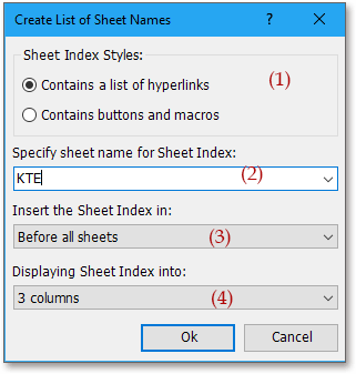
(2)リンクテーブルの名前テキストボックスにデータを入力して、新しいインデックスシートの名前を指定します。
(3) ワークブック内の位置リストで、追加するインデックスシートの配置場所を指定します。
(4) シート名を1 列のリストで表示したい場合は、スパンする行数リストで「1 列」を選択します。
3。「OK」をクリックすると、シート名が一覧表示されます。
ヒント:
1。シート名をクリックするだけで、対応する元のシートに瞬時に移動できます。
2。このリストやシート名は、シートの挿入や削除に対して自動的に更新されません。
3。実際には、相手先のシートにリンクするボタンのリストを作成することも可能です。そのためには、ダイアログボックスでボタンとマクロの作成をオンにするだけです。スクリーンショットをご参照ください:
リンクテーブルの作成方法について詳しくはこちらをクリックしてください。
クリック可能なシート名リストの作成
Kutools for Excel を使用してワークシート名の動的リストを表示する
Kutools for Excel をご利用の場合、ナビゲーションユーティリティを使って、リンク可能なワークシート名をペインに表示することもできます。
Kutools for Excel を無料でインストールした後、以下の手順に従ってください:
1。Kutools > ナビゲーションをクリックします。「ワークブックとシート」をクリックすると、ワークブックとワークシートが表示され、ワークブックを選択するとそのワークシートがナビゲーションペインに表示されます。スクリーンショットを参照してください:
ヒント:
ワークシートが削除または追加された場合は、 をナビゲーションペイン内でクリックして、ワークシート名を更新できます。
ナビゲーション機能の詳細についてはこちらをクリックしてください。
ナビゲーション — シートの一覧表示
最高の Office 業務効率化ツール
| 🤖 | KUTOOLS AI アシスタント:次に基づいてデータ分析を革新します:インテリジェント実行 | コード生成| カスタム数式作成 | データ分析とチャート生成| 拡張機能呼び出し… |
| 人気の機能:検索・ハイライト、または重複をマーキング | 空白行を削除する | データを失うことなく列の結合またはセルを | 数式を使用しない四捨五入... | |
| スーパー LOOKUP:複数条件 VLookup | 複数値 VLookup | 複数シート間 VLookup | ファジーマッチ.... | |
| 高度なドロップダウンリスト:ドロップダウンリストをすばやく作成 | 連動型ドロップダウンリスト | 複数選択可能なドロップダウンリスト.... | |
| 列マネージャー:指定した数の列を追加|列の移動|非表示列の表示状態を切り替え|範囲および列の比較... | |
| 注目の機能:グリッドフォーカス | デザインビュー |強化された数式バー | ワークブックとシートマネージャー | リソースライブラリ(オートテキスト)| 日付ピッカー | ワークシートの統合 | 暗号化/セルの復号化 | リストからメール送信 | スーパーフィルター | 特殊フィルタ(太字のフォントを持つセルをフィルタリング/斜体/取り消し線。。。) 。。。 | |
| トップ15 ツールセット:12 テキストツール(テキストの追加、特定の文字を削除、...)| 50+チャートタイプ(ガントチャート、...)| 40+実用的関数(誕生日に基づいて年齢を計算します、...)| 19 挿入ツール(QR コードを挿入、パスから画像を挿入、...)| 12 変換ツール(単語に変換する、為替レートの変換、...)| 7 結合と分割ツール(高度な行のマージ、セルの分割、...)|さらに多数 |
Kutools for Excel でExcel スキルを強化し、これまでにない効率を体験しましょう。Kutools for Excel は、生産性を高め、時間を大幅に節約できる高度な機能を300 以上提供します。最も必要な機能を今すぐ入手するにはこちらをクリック。。。
Office Tab は Office にタブインターフェースをもたらし、作業を大幅に簡単にします
- Word、Excel、PowerPoint でタブを使った編集と閲覧を有効にします。Publisher、Access、Visio、Project でもご利用いただけます。
- 複数のドキュメントを、新しいウィンドウではなく、同じウィンドウ内の新しいタブで開いたり作成したりできます。
- 日々の生産性を50%も向上させ、毎日数百回ものマウスクリックを削減します!
すべてのKutools アドインが、たった1 つのインストーラーで完結。
Kutools for Officeスイートには、Excel ・Word ・Outlook ・PowerPoint 用のアドインと Office Tab Pro が含まれており、複数の Office アプリを横断して作業するチームに最適です。
- オールインワンスイート— Excel、Word、Outlook、PowerPoint 用アドイン+Office Tab Pro
- インストーラー1 つ、ライセンス1 つ— 数分でセットアップ可能(MSI 対応)
- 連携してさらにパワーアップ— Office アプリ全体で生産性が向上
- 30 日間のフル機能トライアル— 登録不要、クレジットカード不要
- 最高のお得感— 個別アドイン購入よりお得