Excel で行または列の一致項目を VLOOKUP して合計するには？

VLOOKUP 関数と SUM 関数を組み合わせれば、指定された条件に一致する値を素早く探し出し、対応する数値を即座に合計できます。この記事では、Excel で行または列の最初の一致値、あるいはすべての一致値を VLOOKUP で検索して合計する2 つの方法をご紹介します。

数式を使用して、1 行または複数行の一致項目を VLOOKUP して合計する
数式を使用して、列の一致項目を VLOOKUP して合計する
便利なツールで、行または列の一致項目を簡単に VLOOKUP して合計する
VLOOKUP に関するその他のチュートリアル。。。

数式を使用して、1 行または複数行の一致項目を VLOOKUP して合計する

このセクションの数式を使えば、Excel で特定の条件に基づいて最初に一致した1 行（または複数行）の値、あるいはすべての一致値を合計できます。以下の手順に従って操作してください。

1 行で最初に一致した値を VLOOKUP して合計する

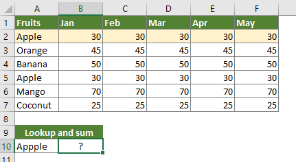
下のスクリーンショットのように果物のテーブルがあり、そのテーブル内で最初に見つかる「Apple」の行にあるすべての対応する値を合計したいとします。この操作を行うには、以下の手順に従ってください。

1．結果を表示する空白セル（ここではセル B10）を選択し、以下の数式をコピーして貼り付け、Ctrl+Shift+Enterキーを押して結果を取得します。

=SUM(VLOOKUP(A10, $A$2:$F$7, {2,3,4,5,6}, FALSE))

注：

• A10は、検索対象の値を含むセルです。
• $A$2:$F$7は、検索値と一致するデータを含むテーブル範囲（ヘッダーを除く）です。
• 数値 {2,3,4,5,6}は、結果値の列がテーブルの2 列目から6 列目までであることを示します。結果列の数が6 を超える場合は、{2,3,4,5,6}を{2,3,4,5,6,7,8,9…}に変更してください。

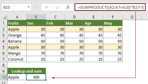
複数行のすべての一致値を VLOOKUP して合計する

上記の数式は、最初に一致した値が含まれる行の値のみを合計します。複数の行にあるすべての一致値を合計したい場合は、以下の手順に従ってください。

1．空白セル（ここではセル B10）を選択し、以下の数式をコピーして貼り付け、Enterキーを押すと、結果が表示されます。

=SUMPRODUCT((A2:A7=A10)*B2:F7)

数式を使用して、列の一致値を VLOOKUP して合計する

このセクションでは、特定の条件に基づいてExcel で列の合計を返す数式をご紹介します。たとえば、下のスクリーンショットのように、果物テーブル内で列タイトル「Jan」を検索し、その列のすべての値を合計する場合です。以下の手順に従って操作してください。

1．空白セルを選択し、以下の数式をコピーして貼り付け、Enterキーを押すと、結果が表示されます。

=SUM(INDEX(B2:F7,0,MATCH(A10,B1:F1,0)))

便利なツールで、行または列の一致項目を簡単に VLOOKUP して合計する

数式が苦手な方には、VLOOKUP と合計機能を搭載したKutools for Excelがおすすめです。この機能を使えば、クリック操作だけで行や列の一致項目を簡単に VLOOKUP して合計できます！

1 行または複数行の最初の一致値、またはすべての一致値を VLOOKUP して合計する

1．Kutools > スーパー LOOKUP > 検索と合計をクリックして、この機能を有効にしてください。スクリーンショットをご覧ください：

2．検索と合計ダイアログボックスで、以下のように設定します。

• 2.1) 検索と合計のタイプを選択してくださいセクションで、行を検索して合計しますオプションを選択します。
• 2.2) 検索値の範囲ボックスで、検索対象の値を含むセルを選択します。
• 2.3) リスト配置エリアボックスで、結果を出力するセルを選択します。
• 2.4) データテーブル範囲ボックスで、列ヘッダーを除いたテーブル範囲を選択します。
• 2.5)オプションセクションで、最初に一致した項目の値だけを合計したい場合は、最初に一致するアイテムの合計結果を返しますオプションを選択してください。すべての一致項目の値を合計したい場合は、すべての一致値の合計を返すオプションをお選びください。
• 2.6) OKボタンをクリックすると、すぐに結果が表示されます。スクリーンショットをご確認ください：

注：列または複数列の最初の一致値、またはすべての一致値を VLOOKUP で合計したい場合は、ダイアログボックスで列を検索して合計しますオプションをオンにして、下のスクリーンショットのように設定してください。

この機能の詳細については、こちらをクリックしてください。

関連記事

最高の Office 業務効率化ツール

🤖	KUTOOLS AI アシスタント：次に基づいてデータ分析を革新します：インテリジェント実行   ｜  コード生成｜  カスタム数式作成  ｜  データ分析とチャート生成｜  拡張機能呼び出し…
	人気の機能：検索・ハイライト、または重複をマーキング   ｜  空白行を削除する   ｜  データを失うことなく列の結合またはセルを   ｜  数式を使用しない四捨五入...
	スーパー LOOKUP：複数条件 VLookup  ｜  複数値 VLookup  ｜   複数シート間 VLookup   ｜   ファジーマッチ....
	高度なドロップダウンリスト：ドロップダウンリストをすばやく作成   ｜  連動型ドロップダウンリスト   ｜  複数選択可能なドロップダウンリスト....
	列マネージャー：指定した数の列を追加｜列の移動｜非表示列の表示状態を切り替え｜範囲および列の比較...
	注目の機能：グリッドフォーカス   ｜  デザインビュー   ｜強化された数式バー   ｜ ワークブックとシートマネージャー   ｜  リソースライブラリ（オートテキスト）｜  日付ピッカー   ｜  ワークシートの統合  ｜  暗号化／セルの復号化   ｜ リストからメール送信   ｜  スーパーフィルター   ｜   特殊フィルタ（太字のフォントを持つセルをフィルタリング／斜体／取り消し線。。。） 。。。
	トップ15 ツールセット：12 テキストツール（テキストの追加、特定の文字を削除、...）｜   50+チャートタイプ（ガントチャート、...）｜   40+実用的関数（誕生日に基づいて年齢を計算します、...）｜   19 挿入ツール（QR コードを挿入、パスから画像を挿入、...）｜   12 変換ツール（単語に変換する、為替レートの変換、...）｜   7 結合と分割ツール（高度な行のマージ、セルの分割、...）｜さらに多数

Kutools はお好みの言語でご利用いただけます。英語、スペイン語、ドイツ語、フランス語、中国語、および40+の他の言語をサポートしています！

Kutools for Excel でExcel スキルを強化し、これまでにない効率を体験しましょう。Kutools for Excel は、生産性を高め、時間を大幅に節約できる高度な機能を300 以上提供します。最も必要な機能を今すぐ入手するにはこちらをクリック。。。

Kutools for Excel の詳細はこちら。。。無料ダウンロード。。。

---

Office Tab は Office にタブインターフェースをもたらし、作業を大幅に簡単にします

• Word、Excel、PowerPoint でタブを使った編集と閲覧を有効にします。Publisher、Access、Visio、Project でもご利用いただけます。
• 複数のドキュメントを、新しいウィンドウではなく、同じウィンドウ内の新しいタブで開いたり作成したりできます。
• 日々の生産性を50％も向上させ、毎日数百回ものマウスクリックを削減します！

Office Tab の詳細はこちら。。。無料ダウンロード。。。

---

すべてのKutools アドインが、たった1 つのインストーラーで完結。

Kutools for Officeスイートには、Excel ・Word ・Outlook ・PowerPoint 用のアドインと Office Tab Pro が含まれており、複数の Office アプリを横断して作業するチームに最適です。

• オールインワンスイート— Excel、Word、Outlook、PowerPoint 用アドイン＋Office Tab Pro
• インストーラー1 つ、ライセンス1 つ— 数分でセットアップ可能（MSI 対応）
• 連携してさらにパワーアップ— Office アプリ全体で生産性が向上
• 30 日間のフル機能トライアル— 登録不要、クレジットカード不要
• 最高のお得感— 個別アドイン購入よりお得

Kutools for Office の詳細はこちら。。。無料ダウンロード。。。