別の列に同じ値が存在する場合、Excelでセルを連結するにはどうすればよいですか？

以下のスクリーンショットに示すように、最初の列の同じ値に基づいて2番目の列のセルを連結したい場合、いくつかの方法があります。この記事では、このタスクを実行するための3つの方法を紹介します。

数式とフィルターを使用して同じ値を持つセルを連結する

次の数式は、ある列の一致する値に基づいて、対応するセルを別の列に連結するのに役立ちます。

1. 2列目の隣にある空白セルを選択し（ここではセルC2を選択）、数式バーに =IF(A2<>A1,B2,C1 & "," & B2) という数式を入力し、Enterキーを押します。

2. 次に、セルC2を選択し、結合したいセルまでフィルハンドルを下にドラッグします。

3. セルD2に =IF(A2<>A3,CONCATENATE(A2,"","",C2,"""),"") という数式を入力し、残りのセルまでフィルハンドルをドラッグします。

4. セルD1を選択し、データ > フィルター をクリックします。スクリーンショットをご覧ください：

5. セルD1のドロップダウン矢印をクリックし、(空白) のチェックボックスをオフにして、OKボタンをクリックします。

これで、最初の列の値が同じ場合、セルが連結されていることが確認できます。

注: 上記の数式を正常に使用するには、列Aの同じ値が連続している必要があります。

Kutools for Excelを使用して、数回のクリックで簡単に同じ値を持つセルを連結する

上記の方法では、2つの補助列を作成し、複数のステップが必要なため、不便かもしれません。より簡単な方法をお探しならば、Kutools for Excelの「高度な行のマージ」ツールの使用を検討してください。このユーティリティを使えば、特定の区切り文字を使用してセルを数回のクリックで連結でき、プロセスが迅速かつ手間なく行えます。

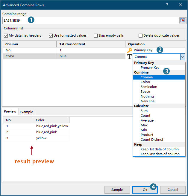
1. Kutools > 結合と分割 > 高度な行のマージ をクリックして、この機能を有効にします。

2. 「高度な行のマージ」ダイアログボックスで、以下を行うだけです：

• 連結したい範囲を選択します；
• 同じ値を持つ列をキーカラムとして設定します。
• セルを結合するための区切り文字を指定します。
• OK をクリックします。

結果

VBAコードを使用して同じ値を持つセルを連結する

VBAコードを使用して、別の列に同じ値が存在する場合、列内のセルを連結することもできます。

1. Alt + F11 キーを押して Microsoft Visual Basic for Applications ウィンドウを開きます。

2. Microsoft Visual Basic for Applications ウィンドウで、挿入 > モジュール をクリックします。次に、以下のコードをモジュールウィンドウにコピーして貼り付けます。

VBAコード：同じ値を持つセルを連結する

Sub ConcatenateCellsIfSameValues()
	Dim xCol As New Collection
	Dim xSrc As Variant
	Dim xRes() As Variant
	Dim I As Long
	Dim J As Long
	Dim xRg As Range
	xSrc    = Range("A1", Cells(Rows.Count, "A").End(xlUp)).Resize(, 2)
	Set xRg = Range("D1")
	On Error Resume Next
	For I = 2 To UBound(xSrc)
		xCol.Add xSrc(I, 1), TypeName(xSrc(I, 1)) & CStr(xSrc(I, 1))
	Next I
	On Error GoTo 0
	ReDim xRes(1 To xCol.Count + 1, 1 To 2)
	xRes(1, 1) = "No"
	xRes(1, 2) = "Combined Color"
	For I = 1 To xCol.Count
		xRes(I + 1, 1) = xCol(I)
		For J = 2 To UBound(xSrc)
			If xSrc(J, 1) = xRes(I + 1, 1) Then
				xRes(I + 1, 2) = xRes(I + 1, 2) & ", " & xSrc(J, 2)
			End If
		Next J
		xRes(I + 1, 2) = Mid(xRes(I + 1, 2), 2)
	Next I
	Set xRg = xRg.Resize(UBound(xRes, 1), UBound(xRes, 2))
	xRg.NumberFormat = "@"
	xRg = xRes
	xRg.EntireColumn.AutoFit
End Sub

注意：

3. コードを実行するために F5 キーを押すと、指定された範囲で連結された結果が得られます。

デモ： Kutools for Excelを使用して、同じ値を持つセルを簡単に連結する

最高のオフィス業務効率化ツール

🤖	Kutools AI Aide：データ分析を革新します。主な機能：Intelligent Execution｜コード生成｜カスタム数式の作成｜データの分析とグラフの生成｜Kutools Functionsの呼び出し……
	人気の機能：重複の検索・ハイライト・重複をマーキング｜空白行を削除｜データを失わずに列またはセルを統合｜丸める……
	スーパーLOOKUP：複数条件でのVLookup｜複数値でのVLookup｜複数シートの検索｜ファジーマッチ……
	高度なドロップダウンリスト：ドロップダウンリストを素早く作成｜連動ドロップダウンリスト｜複数選択ドロップダウンリスト……
	列マネージャー：指定した数の列を追加 ｜列の移動 ｜非表示列の表示/非表示の切替｜ 範囲＆列の比較……
	注目の機能：グリッドフォーカス｜デザインビュー｜強化された数式バー｜ワークブック＆ワークシートの管理｜オートテキスト ライブラリ｜日付ピッカー｜データの統合 ｜セルの暗号化/復号化｜リストで電子メールを送信｜スーパーフィルター｜特殊フィルタ（太字/斜体/取り消し線などをフィルター）……
	トップ15ツールセット：12 種類のテキストツール（テキストの追加、特定の文字を削除など）｜50種類以上のグラフ（ガントチャートなど）｜40種類以上の便利な数式（誕生日に基づいて年齢を計算するなど）｜19 種類の挿入ツール（QRコードの挿入、パスから画像の挿入など）｜12 種類の変換ツール（単語に変換する、通貨変換など）｜7種の統合＆分割ツール（高度な行のマージ、セルの分割など）｜… その他多数

Kutoolsはお好みの言語で利用可能 ― 英語、スペイン語、ドイツ語、フランス語、中国語、その他40以上の言語に対応！

Kutools for ExcelでExcelスキルを強化し、これまでにない効率を体感しましょう。 Kutools for Excelは300以上の高度な機能で生産性向上と保存時間を実現します。最も必要な機能はこちらをクリック...

Kutools for Excelの詳細はこちら... 無料ダウンロード...

---

Office TabでOfficeにタブインターフェースを追加し、作業をもっと簡単に

• Word、Excel、PowerPointでタブによる編集・閲覧を実現。
• 新しいウィンドウを開かず、同じウィンドウの新しいタブで複数のドキュメントを開いたり作成できます。
• 生産性が50%向上し、毎日のマウスクリック数を何百回も削減！

Office Tabの詳細はこちら... 無料ダウンロード...

---

全てのKutoolsアドインを一つのインストーラーで

Kutools for Officeスイートは、Excel、Word、Outlook、PowerPoint用アドインとOffice Tab Proをまとめて提供。Officeアプリを横断して働くチームに最適です。

• オールインワンスイート — Excel、Word、Outlook、PowerPoint用アドインとOffice Tab Proが含まれます
• 1つのインストーラー・1つのライセンス —— 数分でセットアップ完了（MSI対応）
• 一括管理でより効率的 —— Officeアプリ間で快適な生産性を発揮
• 30日間フル機能お試し —— 登録やクレジットカード不要
• コストパフォーマンス最適 —— 個別購入よりお得

Kutools for Officeの詳細はこちら... 無料ダウンロード...