Excel で1 つまたは複数の条件に基づいて一意の値を抽出する

著者Xiaoyang変更日2025-04-10

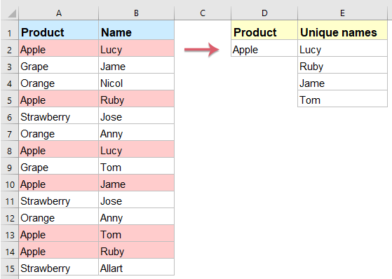
条件に基づいて一意の値を抽出することは、データ分析やレポート作成において非常に重要なタスクです。左側に示されているようなデータ範囲があり、列 A の特定の条件を満たす行に該当する列 B の一意の名前のみをリストしたいとします。このガイドでは、Excel の古いバージョンをご利用の場合でも、最新のExcel 365／2021 の機能をご活用の場合でも、一意の値を効率的に抽出する方法をわかりやすく解説します。

Excel で条件に基づいて一意の値を抽出する

配列数式を使用
Kutools for Excel を使用
数式を使用（Excel 365、Excel 2021 以降）

Excel で複数の条件に基づいて一意の値を抽出する

配列数式を使用
数式を使用（Excel 365、Excel 2021 以降）

Kutools for Excel を使用してセル範囲から一意の値を抽出する

Excel で条件に基づいて一意の値を抽出する

•配列数式を使用して一意の値を縦方向にリストする

この作業を実行するには、複雑な配列数式を適用できます。以下の手順に従って操作してください。

1。抽出結果をリストしたい空白セル（この例ではセル E2）に以下の数式を入力し、Shift キー＋Ctrl キー＋Enter キーを押して、最初の一意な値を取得します。

=IFERROR(INDEX($B$2:$B$15, MATCH(0, IF($D$2=$A$2:$A$15, COUNTIF($E$1:$E1, $B$2:$B$15), ""), 0)),"")

2。次に、フィルハンドルを下方向にドラッグし、空白セルが表示されるまでセル範囲を埋めてください。これにより、特定の条件に基づくすべての一意な値がリストされます（スクリーンショット参照）。

条件に基づき配列数式を使用してExcelで抽出された一意の値のスクリーンショット

注：上記の数式について：B2:B15は抽出元となる一意の値を含む列範囲、A2:A15は条件に基づく列、D2は一意の値をリストするための条件を示し、E1は数式を入力したセルの上のセルです。

•Kutools for Excel を使用して一意の値を1 つのセルに抽出および表示する

Kutools for Excel を使えば、数式を覚える必要なく、大規模なデータセットを手間なく処理し、一意の値を素早く抽出して1 つのセルに表示できます。

Kutools for Excelは300 以上の高度な機能を提供し、複雑な作業を効率化して、創造性と生産性を高めます。AI 機能と統合されたKutools は、正確にタスクを自動化し、データ管理を簡単にします。Kutools for Excel の詳細情報。。。 無料トライアル。。。

Kutools for Excel をインストール後、以下の手順に従って操作してください。

「Kutools」＞「スーパー LOOKUP」＞「一対多の検索（複数の結果を返す）」をクリックしてダイアログボックスを開き、以下の手順に従って操作を指定してください。

それぞれのテキストボックスで、「リスト配置エリア」と「検索値の範囲」を選択してください。
使用するテーブルの範囲を選択してください。
「キーカラム」および「返すカラム」のドロップダウンから、それぞれ対応するカラムを指定してください。
最後に、「OK」ボタンをクリックしてください。

結果：

条件に基づくすべてのユニークな名前が1 つのセルに抽出されました（スクリーンショット参照）。
Kutoolsによって単一セルに抽出された一意の値のスクリーンショット

•Excel 365、Excel 2021 以降の数式を使用して一意の値を縦方向にリストする

Excel 365 およびExcel 2021 では、UNIQUE 関数や FILTER 関数を使えば、一意の値を簡単に抽出できます。

空白セルに次の数式を入力して Enter キーを押すと、すべての重複しない名前が一括で縦方向に表示されます。

=UNIQUE(FILTER(B2:B15, A2:A15=D2))

UNIQUE関数によって抽出された一意の値のスクリーンショット

この数式の説明：

FILTER(B2:B15, A2:A15=D2):
- FILTERB2:B15 のデータをフィルターします。
- A2:A15=D2A2:A15 の値が D2 の値と一致するかどうかを確認し、この条件を満たす行のみが結果に含まれます。
UNIQUE(...):
フィルター結果に一意の値のみが含まれるようにします。

Excel で複数の条件に基づいて一意の値を抽出する

•配列数式を使用して一意の値を縦方向にリストする

2 つの条件に基づいて一意の値を抽出したい場合は、次の配列数式が役立ちます。以下の手順に従って操作してください。

1。一意の値をリストしたい空白セル（この例ではセル G2）に以下の数式を入力し、Shift キー＋Ctrl キー＋Enter キーを押して、最初の一意の値を取得します。

=IFERROR(INDEX($C$2:$C$15,MATCH(0,COUNTIF(G1:$G$1,$C$2:$C$15)+IF($A$2:$A$15<>$E$2,1,0)+IF($B$2:$B$15<>$F$2,1,0),0)),"")

2。次に、フィルハンドルを下方向にドラッグし、空白セルが表示されるまでセル範囲を埋めます。これにより、特定の2 つの条件に基づくすべての一意な値がリストされます（スクリーンショット参照）。

配列数式を使用して複数の条件に基づきExcelで抽出された一意の値を示すスクリーンショット

注：上記の数式において：C2:C15は、抽出したい一意の値を含む列範囲です。A2:A15およびE2は、一意の値を抽出するための最初の条件範囲です。B2:B15およびF2は、一意の値を抽出するための2 番目の条件範囲であり、G1は入力した数式の上のセルです。

•Excel 365、Excel 2021 以降を使用して一意の値を縦方向にリストする

最新版のExcel では、複数の条件に基づいて一意の値を抽出するのが格段に簡単になりました。

空白セルに次の数式を入力して Enter キーを押すと、すべての重複しない名前が一括で縦方向に表示されます。

=UNIQUE(FILTER(C2:C15, (A2:A15=E2) * (B2:B15=F2)))

UNIQUE関数によってさらに多くの条件に基づき抽出された一意の値のスクリーンショット

この数式の説明：

FILTER(C2:C15, (A2:A15=E2) * (B2:B15=F2)):
- FILTERC2:C15 のデータをフィルターします。
- (A2:A15=E2) 列 A の値が E2 の値と一致するか確認します。
- (B2:B15=F2) 列 B の値が F2 の値と一致するか確認します。
- *2 つの条件を AND 論理で組み合わせます。つまり、行が結果に含まれるには、両方の条件を満たす必要があります。
UNIQUE(...):
フィルター結果から重複を除外し、出力には一意の値のみを含めるようにします。

Kutools for Excel を使用してセル範囲から一意の値を抽出する

場合によっては、セル範囲から一意の値を抽出したいこともあるでしょう。そんなときは、便利なツール「Kutools for Excel」がおすすめです。「指定された範囲から一意の値を持つセルを抽出します（最初の重複を含む）」機能を使えば、一意の値を素早く簡単に抽出できます。

1。結果を出力したいセルをクリックしてください。（)注：最初の行のセルは選択しないでください。）

2。次に、「Kutools」＞「関数ヘルパー」＞「関数ヘルパー」をクリックしてください（スクリーンショット参照）。

ExcelのKutoolsタブで「数式ヘルパー」オプションが強調表示されているスクリーンショット

3。「関数ヘルパー」ダイアログボックスで、次の操作を行ってください。

「関数の種類」ドロップダウンリストで「テキスト」オプションを選択してください。
次に、「数式の選択」リストボックスから「指定された範囲から一意の値を持つセルを抽出します（最初の重複を含む）」を選択してください。
右側の「引数の入力」セクションで、一意の値を抽出したいセル範囲を指定してください。

Excelの「数式ヘルパー」ダイアログで「一意の値を持つセルを抽出」オプションが選択されているスクリーンショット

4。「OK」ボタンをクリックすると、セルに最初の結果が表示されます。その後、そのセルを選択してフィルハンドルをドラッグし、空白セルが現れるまで一意の値をすべてリストしてください（スクリーンショット参照）。

Kutoolsの「一意の値を持つセルを抽出」機能を使用してExcelに出力された一意の値を示すスクリーンショット

Excel で条件に基づいて一意の値を抽出することは、効率的なデータ分析に欠かせないタスクです。Excel のバージョンや目的に応じて、複数の方法から最適なものを選べば、スピーディーかつ正確に一意の値を抽出できます。さらに多くのExcel テクニックやヒントを知りたい方は、当社のウェブサイトに数千ものチュートリアルが掲載されています。

リスト内の一意および個別の値の数をカウントする
重複項目を含む長い値のリストがあると仮定します。その際、列内で「一意の値」（リスト内に1 回だけ出現する値）または「個別の値」（リスト内のすべての異なる値、つまり一意の値＋各重複値の最初の出現分）の数をカウントしたい場合があるでしょう（左のスクリーンショット参照）。本記事では、Excel でこうした作業を効率的に処理する方法をご紹介します。

Excel で条件に基づいて一意の値を合計する
たとえば、「名前」と「注文」列を含むデータ範囲があるとします。このとき、以下のスクリーンショットのように、「名前」列に基づいて「注文」列の一意の値のみを合計したい場合、Excel でこのタスクを素早く簡単に実現するにはどうすればよいでしょうか？

別の列の一意の値に基づいて1 つの列のセルを行方向に転置する
2 列からなるデータ範囲があり、そのうち1 列のセルを、別の列の一意の値に基づいて行方向に転置し、次のような結果を得たいと考えています。Excel でこの課題を解決する良い方法はありますか？

Excel で一意の値を連結する
重複データを含む長い値のリストがあるとします。このとき、一意の値だけを抽出して、それらを1 つのセルにカンタンかつスピーディーに連結するには、Excel でどうすればよいでしょうか？

最高の Office 業務効率化ツール

🤖	KUTOOLS AI アシスタント：次に基づいてデータ分析を革新します：インテリジェント実行｜コード生成｜カスタム数式作成｜データ分析とチャート生成｜拡張機能呼び出し…
	人気の機能：検索・ハイライト、または重複をマーキング｜空白行を削除する｜データを失うことなく列の結合またはセルを｜数式を使用しない四捨五入...
	スーパー LOOKUP：複数条件 VLookup ｜複数値 VLookup ｜複数シート間 VLookup ｜ファジーマッチ....
	高度なドロップダウンリスト：ドロップダウンリストをすばやく作成｜連動型ドロップダウンリスト｜複数選択可能なドロップダウンリスト....
	列マネージャー：指定した数の列を追加｜列の移動｜非表示列の表示状態を切り替え｜範囲および列の比較...
	注目の機能：グリッドフォーカス｜デザインビュー｜強化された数式バー｜ワークブックとシートマネージャー｜リソースライブラリ（オートテキスト）｜日付ピッカー｜ワークシートの統合｜暗号化／セルの復号化｜リストからメール送信｜スーパーフィルター｜特殊フィルタ（太字のフォントを持つセルをフィルタリング／斜体／取り消し線。。。）。。。
	トップ15 ツールセット：12 テキストツール（テキストの追加、特定の文字を削除、...）｜ 50+チャートタイプ（ガントチャート、...）｜ 40+実用的関数（誕生日に基づいて年齢を計算します、...）｜ 19 挿入ツール（QR コードを挿入、パスから画像を挿入、...）｜ 12 変換ツール（単語に変換する、為替レートの変換、...）｜ 7 結合と分割ツール（高度な行のマージ、セルの分割、...）｜さらに多数

Kutools はお好みの言語でご利用いただけます。英語、スペイン語、ドイツ語、フランス語、中国語、および40+の他の言語をサポートしています！

Kutools for Excel でExcel スキルを強化し、これまでにない効率を体験しましょう。Kutools for Excel は、生産性を高め、時間を大幅に節約できる高度な機能を300 以上提供します。最も必要な機能を今すぐ入手するにはこちらをクリック。。。

Kutools for Excel の詳細はこちら。。。無料ダウンロード。。。

Office Tab は Office にタブインターフェースをもたらし、作業を大幅に簡単にします

Word、Excel、PowerPoint でタブを使った編集と閲覧を有効にします。Publisher、Access、Visio、Project でもご利用いただけます。
複数のドキュメントを、新しいウィンドウではなく、同じウィンドウ内の新しいタブで開いたり作成したりできます。
日々の生産性を50％も向上させ、毎日数百回ものマウスクリックを削減します！