特定のテキストを含むセルがある場合、別のセルに値を返すにはどうすればよいですか?
下記の例のように、セルE6に「Yes」という値が含まれている場合、セルF6には自動的に「Approve」という値が入力されます。「Yes」を「No」または「Neutrality」に変更すると、F6の値は即座に「Deny」または「Reconsider」に変わります。これを実現するにはどうすればよいでしょうか?この記事では、いくつかの有用な方法を紹介し、簡単に解決するお手伝いをします。

異なるテキストを含むセルがある場合、別のセルに値を返すために数式を使用する
異なるテキストを含むセルがある場合、数回のクリックで簡単に別のセルに値を返す
特定のテキストを含むセルがある場合、別のセルに値を返すために数式を使用する
特定のテキストを含むセルがある場合、別のセルに値を返すには、次の数式を試してください。 例えば、B5に「Yes」が含まれている場合、「Approve」をD5に返し、そうでない場合は「No qualify」を返します。以下のように操作してください。
D5を選択し、以下の数式をコピーして貼り付け、「Enter」キーを押します。スクリーンショットをご覧ください:
数式: 特定のテキストを含むセルがある場合、別のセルに値を返す
=IF(ISNUMBER(SEARCH("Yes",B5)),"Approve","No qualify")注意:
1. 数式において、「Yes」、「B5」、「approve」、「No qualify」は、セルB5に「Yes」というテキストが含まれている場合、指定されたセルには「approve」というテキストが入力され、そうでなければ「No qualify」が入力されることを示しています。必要に応じてこれらを変更できます。
2. 指定されたセルの値に基づいて他のセル(例えばK8やK9)から値を返すには、次の数式を使用してください:
=IF(ISNUMBER(SEARCH("Yes",B5)),K8,K9)
特定の列のセルの値に基づいて、選択範囲内の行全体または行全体を選択する方法:
「Kutools for Excel」の「特定のセルを選択」機能は、Excelの特定の列にある特定のセルの値に基づいて、選択範囲内の行全体または行全体を迅速に選択するのに役立ちます。

Kutools for Excel - 必要なツールを300以上搭載し、Excelの機能を大幅に強化します。永久に無料で利用できるAI機能もお楽しみください!今すぐ入手
異なるテキストを含むセルがある場合、別のセルに値を返すために数式を使用する
このセクションでは、セルに異なるテキストが含まれている場合、別のセルに値を返すための数式をご紹介します。
1. 特定の値と返される値をそれぞれ2つの列に分けて配置した表を作成する必要があります。スクリーンショットをご覧ください:

2. 値を返すための空白セルを選択し、以下の数式を入力して「Enter」キーを押して結果を得ます。スクリーンショットをご覧ください:
数式: 異なるテキストを含むセルがある場合、別のセルに値を返す
=VLOOKUP(E6,B5:C7,2,FALSE)注意:
数式において、E6は返される値に基づく特定の値を含むセルであり、B5:C7は特定の値と返される値を含む列範囲です。数字の2は、テーブル範囲の2番目の列に返される値があることを意味します。
これで、E6の値を特定のものに変更すると、その対応する値が即座にF6に返されます。
異なるテキストを含むセルがある場合、数回のクリックで簡単に別のセルに値を返す
実際、上記の問題をもっと簡単な方法で解決できます。「Kutools for Excel」の「範囲内でデータを検索する」機能を使えば、数式を覚えることなく数回のクリックでそれを実現できます。
1. 上記の方法と同じように、特定の値と返される値をそれぞれ2つの列に分けて配置した表を作成する必要があります。
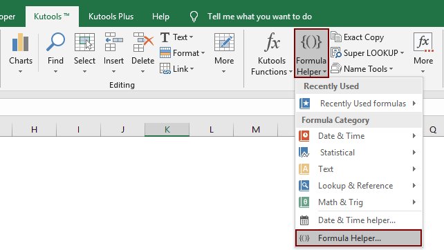
2. 結果を出力するための空白セルを選択します(ここではF6を選択)、そして「Kutools」>「関数ヘルパー」>「関数ヘルパー」をクリックします。スクリーンショットをご覧ください:
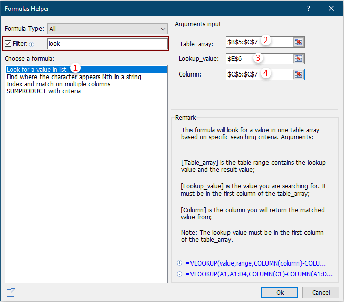
3. 「関数ヘルパー」ダイアログボックスで、次のように設定してください:
- 3.1 「関数を選択」ボックスで、「範囲内でデータを検索する」を見つけて選択します;
ヒント: 「フィルター」ボックスをチェックし、テキストボックスに特定の単語を入力して数式を素早くフィルタリングできます。 - 3.2 「テーブル範囲」ボックスで、ステップ1で作成したヘッダーなしの表を選択します;
- 3.2 「検索値」ボックスで、返される値に基づく特定の値を含むセルを選択します;
- 3.3 「列」ボックスで、一致する値を返す列を指定します。または、必要に応じて直接列番号をテキストボックスに入力することもできます。
- 3.4 「OK」ボタンをクリックします。スクリーンショットをご覧ください:

これで、E6の値を特定のものに変更すると、その対応する値が即座にF6に返されます。以下の結果をご覧ください:

Kutools for Excel - 必要なツールを300以上搭載し、Excelの機能を大幅に強化します。永久に無料で利用できるAI機能もお楽しみください!今すぐ入手
最高のオフィス業務効率化ツール
| 🤖 | Kutools AI Aide:データ分析を革新します。主な機能:Intelligent Execution|コード生成|カスタム数式の作成|データの分析とグラフの生成|Kutools Functionsの呼び出し…… |
| 人気の機能:重複の検索・ハイライト・重複をマーキング|空白行を削除|データを失わずに列またはセルを統合|丸める…… | |
| スーパーLOOKUP:複数条件でのVLookup|複数値でのVLookup|複数シートの検索|ファジーマッチ…… | |
| 高度なドロップダウンリスト:ドロップダウンリストを素早く作成|連動ドロップダウンリスト|複数選択ドロップダウンリスト…… | |
| 列マネージャー:指定した数の列を追加 |列の移動 |非表示列の表示/非表示の切替| 範囲&列の比較…… | |
| 注目の機能:グリッドフォーカス|デザインビュー|強化された数式バー|ワークブック&ワークシートの管理|オートテキスト ライブラリ|日付ピッカー|データの統合 |セルの暗号化/復号化|リストで電子メールを送信|スーパーフィルター|特殊フィルタ(太字/斜体/取り消し線などをフィルター)…… | |
| トップ15ツールセット:12 種類のテキストツール(テキストの追加、特定の文字を削除など)|50種類以上のグラフ(ガントチャートなど)|40種類以上の便利な数式(誕生日に基づいて年齢を計算するなど)|19 種類の挿入ツール(QRコードの挿入、パスから画像の挿入など)|12 種類の変換ツール(単語に変換する、通貨変換など)|7種の統合&分割ツール(高度な行のマージ、セルの分割など)|… その他多数 |
Kutools for ExcelでExcelスキルを強化し、これまでにない効率を体感しましょう。 Kutools for Excelは300以上の高度な機能で生産性向上と保存時間を実現します。最も必要な機能はこちらをクリック...
Office TabでOfficeにタブインターフェースを追加し、作業をもっと簡単に
- Word、Excel、PowerPointでタブによる編集・閲覧を実現。
- 新しいウィンドウを開かず、同じウィンドウの新しいタブで複数のドキュメントを開いたり作成できます。
- 生産性が50%向上し、毎日のマウスクリック数を何百回も削減!
全てのKutoolsアドインを一つのインストーラーで
Kutools for Officeスイートは、Excel、Word、Outlook、PowerPoint用アドインとOffice Tab Proをまとめて提供。Officeアプリを横断して働くチームに最適です。
- オールインワンスイート — Excel、Word、Outlook、PowerPoint用アドインとOffice Tab Proが含まれます
- 1つのインストーラー・1つのライセンス —— 数分でセットアップ完了(MSI対応)
- 一括管理でより効率的 —— Officeアプリ間で快適な生産性を発揮
- 30日間フル機能お試し —— 登録やクレジットカード不要
- コストパフォーマンス最適 —— 個別購入よりお得