メインコンテンツへスキップ

Excelのセル値に基づいて図形の色を変更するにはどうすればよいですか?

特定のセル値に基づいて形状の色を変更することは、Excelで興味深いタスクになる場合があります。たとえば、A1のセル値が100未満の場合、形状の色は赤になり、A1が100より大きく200より小さい場合、形状の色は黄色で、A1が200を超えると、次のスクリーンショットのように形状の色が緑色になります。 セルの値に基づいて形状の色を変更するために、この記事では方法を紹介します。

docチェンジシェイプカラー1

VBAコードを使用してセル値に基づいて形状の色を変更する


矢印青い右バブル VBAコードを使用してセル値に基づいて形状の色を変更する

以下のVBAコードは、セルの値に基づいて形状の色を変更するのに役立ちます。次のようにしてください。

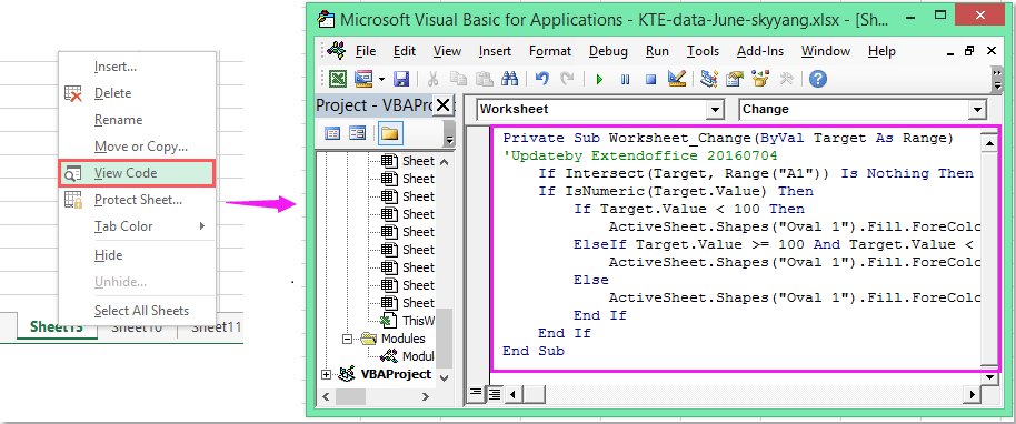
1。 図形の色を変更するシートタブを右クリックして、 コードを表示 コンテキストメニューから、ポップアウトで アプリケーション向け Microsoft Visual Basic ウィンドウの場合は、次のコードをコピーして空白に貼り付けてください モジュール 窓。

VBAコード:セルの値に基づいて形状の色を変更します。

Private Sub Worksheet_Change(ByVal Target As Range)
'Updateby Extendoffice 20160704
    If Intersect(Target, Range("A1")) Is Nothing Then Exit Sub
    If IsNumeric(Target.Value) Then
        If Target.Value < 100 Then
            ActiveSheet.Shapes("Oval 1").Fill.ForeColor.RGB = vbRed
        ElseIf Target.Value >= 100 And Target.Value < 200 Then
            ActiveSheet.Shapes("Oval 1").Fill.ForeColor.RGB = vbYellow
        Else
            ActiveSheet.Shapes("Oval 1").Fill.ForeColor.RGB = vbGreen
        End If
    End If
End Sub

docチェンジシェイプカラー2

2。 次に、セルA1に値を入力すると、定義したセル値で図形の色が変更されます。

Note:上記のコードでは、 A1 形状の色が変更されるセルの値は、 オーバル1 は挿入した形状の形状名です。必要に応じて変更できます。

最高のオフィス生産性向上ツール

🤖 Kutools AI アシスタント: 以下に基づいてデータ分析に革命をもたらします。 インテリジェントな実行   |  コードを生成  |  カスタム数式の作成  |  データを分析してグラフを生成する  |  Kutools関数を呼び出す...
人気の機能: 重複を検索、強調表示、または識別する   |  空白行を削除する   |  データを失わずに列またはセルを結合する   |   数式なしのラウンド ...
スーパールックアップ: 複数の基準の VLookup    複数の値の VLookup  |   複数のシートにわたる VLookup   |   ファジールックアップ ....
詳細ドロップダウン リスト: ドロップダウンリストを素早く作成する   |  依存関係のドロップダウン リスト   |  複数選択のドロップダウンリスト ....
列マネージャー: 特定の数の列を追加する  |  列の移動  |  Toggle 非表示列の表示ステータス  |  範囲と列の比較 ...
注目の機能: グリッドフォーカス   |  デザインビュー   |   ビッグフォーミュラバー    ワークブックとシートマネージャー   |  リソースライブラリ (自動テキスト)   |  日付ピッカー   |  ワークシートを組み合わせる   |  セルの暗号化/復号化    リストごとにメールを送信する   |  スーパーフィルター   |   特殊フィルター (太字/斜体/取り消し線をフィルター...) ...
上位 15 のツールセット12 テキスト ツール (テキストを追加, 文字を削除する、...)   |   50+ チャート 種類 (ガントチャート、...)   |   40+ 実用的 (誕生日に基づいて年齢を計算する、...)   |   19 挿入 ツール (QRコードを挿入, パスから画像を挿入、...)   |   12 変換 ツール (数字から言葉へ, 通貨の換算、...)   |   7 マージ&スプリット ツール (高度な結合行, 分割セル、...)   |   ... もっと

Kutools for Excel で Excel スキルを強化し、これまでにない効率を体験してください。 Kutools for Excelは、生産性を向上させ、時間を節約するための300以上の高度な機能を提供します。  最も必要な機能を入手するにはここをクリックしてください...

説明


Officeタブは、タブ付きのインターフェイスをOfficeにもたらし、作​​業をはるかに簡単にします

  • Word、Excel、PowerPointでタブ付きの編集と読み取りを有効にする、パブリッシャー、アクセス、Visioおよびプロジェクト。
  • 新しいウィンドウではなく、同じウィンドウの新しいタブで複数のドキュメントを開いて作成します。
  • 生産性を 50% 向上させ、毎日何百回もマウス クリックを減らすことができます!
Comments (22)
Rated 4 out of 5 · 1 ratings
This comment was minimized by the moderator on the site
how would be the VBA code to paint several autoforms according to a range of data?
the values are in column B and I have 20 autoforms.
This comment was minimized by the moderator on the site
Como faço para para variar as cores da forma se minha opções for em formato de texto, como "Sim" e "Não"?
This comment was minimized by the moderator on the site
Hello, Emilly
To solve your problem, please apply the below code:
Private Sub Worksheet_Change(ByVal Target As Range)
If Range("A1") = "Yes" Then
ActiveSheet.Shapes("Oval 1").Fill.ForeColor.RGB = vbRed
Else
If Range("A1") = "No" Then
ActiveSheet.Shapes("Oval 1").Fill.ForeColor.RGB = vbGreen
End If
End If
End Sub


Please have a try, hope it can help you!
This comment was minimized by the moderator on the site
Hi Skyyang,

I tried the original VBA code and got it to work, although it would not activate actively when the cell changed. Today the code is not working and I also tried your more simplistic code and still did not work. The only thing that changed is that I copied the worksheet which contained the code that worked. Would this then result in it not working?
This comment was minimized by the moderator on the site
Hola, excelente ejemplo.
Pero como seria si tengo una forma y quiero ir coloreado poco a poco dependiendo del valor ejemplo:
Si el valor es 50%
Seia mitad roja y mitad verde
Pero que se vaya llenando según el porcentaje vaya aumentando
Rated 4 out of 5
This comment was minimized by the moderator on the site
I am new to VBAs and am struggling with something. I need to have 9 different cells A1-A9 change the colour of 9 different objects. Objects are cubes 1-9. Just to clarify, each cell is to change just one object A1-Cube 1, etc. Red if it fails to meet the value and green if it exceeds the value. The pass/fail value can change so instead of having the value in the VBA I need it to reference cell A10 which has the pass/fail value. Any chance someone could through out a sample code for me to work with.

Thanks
This comment was minimized by the moderator on the site
Great solution! How can I do if I have more than 1 oval in the worksheet which the colors change according to the value input say in A1, B1,C1? Thanks in advance for your reply! 
This comment was minimized by the moderator on the site
Hello mnsosa,Glad to help. Please copy and paste the below VBA code into the blank Module window.
Sub TestMacro2()
Dim dblHt As Double
Dim rngC As Range
Dim lngr As Long
Dim dblMargin As Double
Dim lngSR As Long

lngSR = 2 'Row where the data starts

dblMargin = 6 ' Distance between shapes

'On Error Resume Next
ActiveSheet.Shapes.SelectAll
Selection.Delete
On Error GoTo 0


dblHt = Rows(lngSR).Height * 4

For lngr = lngSR To Cells(lngSR, "A").End(xlDown).Row
ActiveSheet.Shapes.AddShape(msoShapeOval, _
Cells(lngSR, "D").Left + ((lngr - lngSR) Mod 4) * dblHt + dblMargin, _
Cells(lngSR, "D").Top + Int((lngr - lngSR) / 4) * dblHt + dblMargin, _
dblHt - 2 * dblMargin, _
dblHt - 2 * dblMargin).Select
Selection.Name = "Round" & Cells(lngr, "A").Address
Selection.ShapeRange.TextFrame2.VerticalAnchor = msoAnchorMiddle
Selection.ShapeRange(1).TextFrame2.TextRange.Characters.Text = Cells(lngr, "A").Value
With Selection.ShapeRange(1).TextFrame2.TextRange.Characters(1, 2).ParagraphFormat
.FirstLineIndent = 0
.Alignment = msoAlignCenter
End With
With Selection.ShapeRange(1).TextFrame2.TextRange.Characters(1, 2).Font
.Bold = msoTrue
.Fill.Visible = msoTrue
.Fill.ForeColor.ObjectThemeColor = msoThemeColorText1
.Fill.ForeColor.TintAndShade = 0
.Fill.ForeColor.Brightness = 0
.Fill.Transparency = 0
.Fill.Solid
.Size = 12
End With
With Selection.ShapeRange.Fill
.Visible = msoTrue
If Cells(lngr, "A").Value > 70 Then
.ForeColor.RGB = RGB(0, 176, 80)
ElseIf Cells(lngr, "A").Value >= 40 Then
.ForeColor.RGB = RGB(255, 255, 70)
Else
.ForeColor.RGB = RGB(255, 0, 0)
End If
.Transparency = 0
.Solid
End With
Next lngr
Range("A1").Select
End Sub

After you run the VBA code above, you will see multiple shapes are generated, and the colors of these shapes are changed according to the VBA.Please see my screenshot. Hope it can help. Have a nice day.Sincerely,Mandy
This comment was minimized by the moderator on the site
¿Cómo hacemos si tenemos más de 1 Oval en la hoja de trabajo cuyos colores cambian de acuerdo con el valor ingresado, por ejemplo, en A1, B1, C1...? Mil gracias por su ayuda!

This comment was minimized by the moderator on the site
Hello María Noel,
Glad to help. Please copy and paste the below VBA code into the blank Module window.

Sub TestMacro2()
Dim dblHt As Double
Dim rngC As Range
Dim lngr As Long
Dim dblMargin As Double
Dim lngSR As Long

lngSR = 2 'Row where the data starts

dblMargin = 6 ' Distance between shapes

'On Error Resume Next
ActiveSheet.Shapes.SelectAll
Selection.Delete
On Error GoTo 0


dblHt = Rows(lngSR).Height * 4

For lngr = lngSR To Cells(lngSR, "A").End(xlDown).Row
ActiveSheet.Shapes.AddShape(msoShapeOval, _
Cells(lngSR, "D").Left + ((lngr - lngSR) Mod 4) * dblHt + dblMargin, _
Cells(lngSR, "D").Top + Int((lngr - lngSR) / 4) * dblHt + dblMargin, _
dblHt - 2 * dblMargin, _
dblHt - 2 * dblMargin).Select
Selection.Name = "Round" & Cells(lngr, "A").Address
Selection.ShapeRange.TextFrame2.VerticalAnchor = msoAnchorMiddle
Selection.ShapeRange(1).TextFrame2.TextRange.Characters.Text = Cells(lngr, "A").Value
With Selection.ShapeRange(1).TextFrame2.TextRange.Characters(1, 2).ParagraphFormat
.FirstLineIndent = 0
.Alignment = msoAlignCenter
End With
With Selection.ShapeRange(1).TextFrame2.TextRange.Characters(1, 2).Font
.Bold = msoTrue
.Fill.Visible = msoTrue
.Fill.ForeColor.ObjectThemeColor = msoThemeColorText1
.Fill.ForeColor.TintAndShade = 0
.Fill.ForeColor.Brightness = 0
.Fill.Transparency = 0
.Fill.Solid
.Size = 12
End With
With Selection.ShapeRange.Fill
.Visible = msoTrue
If Cells(lngr, "A").Value > 70 Then
.ForeColor.RGB = RGB(0, 176, 80)
ElseIf Cells(lngr, "A").Value >= 40 Then
.ForeColor.RGB = RGB(255, 255, 70)
Else
.ForeColor.RGB = RGB(255, 0, 0)
End If
.Transparency = 0
.Solid
End With
Next lngr
Range("A1").Select
End Sub

After you run the VBA code above, you will see multiple shapes are generated, and the colors of these shapes are changed according to the VBA.
Please see my screenshot. Hope it can help. Have a nice day.
Sincerely,
Mandy
This comment was minimized by the moderator on the site
Hi... excellent solution... but how do I apply it to multiple shapes based on the corresponding values of a range of cells. Many thanks in advance for your help.
This comment was minimized by the moderator on the site
Hello Ryan,
Glad to help. Please copy and paste the below VBA code into the blank Module window.

Sub TestMacro2()
Dim dblHt As Double
Dim rngC As Range
Dim lngr As Long
Dim dblMargin As Double
Dim lngSR As Long

lngSR = 2 'Row where the data starts

dblMargin = 6 ' Distance between shapes

'On Error Resume Next
ActiveSheet.Shapes.SelectAll
Selection.Delete
On Error GoTo 0


dblHt = Rows(lngSR).Height * 4

For lngr = lngSR To Cells(lngSR, "A").End(xlDown).Row
ActiveSheet.Shapes.AddShape(msoShapeOval, _
Cells(lngSR, "D").Left + ((lngr - lngSR) Mod 4) * dblHt + dblMargin, _
Cells(lngSR, "D").Top + Int((lngr - lngSR) / 4) * dblHt + dblMargin, _
dblHt - 2 * dblMargin, _
dblHt - 2 * dblMargin).Select
Selection.Name = "Round" & Cells(lngr, "A").Address
Selection.ShapeRange.TextFrame2.VerticalAnchor = msoAnchorMiddle
Selection.ShapeRange(1).TextFrame2.TextRange.Characters.Text = Cells(lngr, "A").Value
With Selection.ShapeRange(1).TextFrame2.TextRange.Characters(1, 2).ParagraphFormat
.FirstLineIndent = 0
.Alignment = msoAlignCenter
End With
With Selection.ShapeRange(1).TextFrame2.TextRange.Characters(1, 2).Font
.Bold = msoTrue
.Fill.Visible = msoTrue
.Fill.ForeColor.ObjectThemeColor = msoThemeColorText1
.Fill.ForeColor.TintAndShade = 0
.Fill.ForeColor.Brightness = 0
.Fill.Transparency = 0
.Fill.Solid
.Size = 12
End With
With Selection.ShapeRange.Fill
.Visible = msoTrue
If Cells(lngr, "A").Value > 70 Then
.ForeColor.RGB = RGB(0, 176, 80)
ElseIf Cells(lngr, "A").Value >= 40 Then
.ForeColor.RGB = RGB(255, 255, 70)
Else
.ForeColor.RGB = RGB(255, 0, 0)
End If
.Transparency = 0
.Solid
End With
Next lngr
Range("A1").Select
End Sub

After you run the VBA code above, you will see multiple shapes are generated, and the colors of these shapes are changed according to the VBA.
Please see my screenshot. Hope it can help. Have a nice day.
Sincerely,
Mandy
This comment was minimized by the moderator on the site
How do I make the private sub to read the result from the AVERAGE(C1,C5,C9) calculation?

Sub only works with numeric values; any thoughts and suggestions are greatly appreciated.
This comment was minimized by the moderator on the site
Hello Cesare,How are you? I notice that the VBA code can work with the AVERAGE(number, number...) calculation. But the trick is that every time you change the values in the calculation, you need to double-click the formula in the cell to make the VBA work again. 
For example, In cell A1, after we input the formula is =AVERAGE(C2:D3), the VBA works and changes the color of the shape accordingly. Please see screenshot 1. <span style="letter-spacing: 0.2px; color: inherit; font-family: inherit; font-style: inherit; font-variant-ligatures: inherit; font-variant-caps: inherit; font-weight: inherit;">C2:D3, the returned result in cell A1 changes, but the shape color hasn't been changed yet. In this case, we need to double click the formula in cell A1 to make the VBA work. Then the shape color will be changed accordingly. Please see screenshots 2 and 3.</span>
This comment was minimized by the moderator on the site
Thanks for this which is really useful.

I now want to use it with a pivot table on another worksheet which controls the data on the sheet with the shapes that I want to change colour. However, when I change the selection on the pivot table the data on the worksheet with the shapes is updated but the code does not run so the shapes do not change colour

If I manually change the values the code runs and the colour of the shapes is updated.

Question: what do i need to add to the code above to allow it to run automatically?
This comment was minimized by the moderator on the site
How can this be applied if you have multiple shape in the same worksheet?
This comment was minimized by the moderator on the site
Hello Yasir,
Glad to help. Please copy and paste the below VBA code into the blank Module window.

Sub TestMacro2()
Dim dblHt As Double
Dim rngC As Range
Dim lngr As Long
Dim dblMargin As Double
Dim lngSR As Long

lngSR = 2 'Row where the data starts

dblMargin = 6 ' Distance between shapes

'On Error Resume Next
ActiveSheet.Shapes.SelectAll
Selection.Delete
On Error GoTo 0


dblHt = Rows(lngSR).Height * 4

For lngr = lngSR To Cells(lngSR, "A").End(xlDown).Row
ActiveSheet.Shapes.AddShape(msoShapeOval, _
Cells(lngSR, "D").Left + ((lngr - lngSR) Mod 4) * dblHt + dblMargin, _
Cells(lngSR, "D").Top + Int((lngr - lngSR) / 4) * dblHt + dblMargin, _
dblHt - 2 * dblMargin, _
dblHt - 2 * dblMargin).Select
Selection.Name = "Round" & Cells(lngr, "A").Address
Selection.ShapeRange.TextFrame2.VerticalAnchor = msoAnchorMiddle
Selection.ShapeRange(1).TextFrame2.TextRange.Characters.Text = Cells(lngr, "A").Value
With Selection.ShapeRange(1).TextFrame2.TextRange.Characters(1, 2).ParagraphFormat
.FirstLineIndent = 0
.Alignment = msoAlignCenter
End With
With Selection.ShapeRange(1).TextFrame2.TextRange.Characters(1, 2).Font
.Bold = msoTrue
.Fill.Visible = msoTrue
.Fill.ForeColor.ObjectThemeColor = msoThemeColorText1
.Fill.ForeColor.TintAndShade = 0
.Fill.ForeColor.Brightness = 0
.Fill.Transparency = 0
.Fill.Solid
.Size = 12
End With
With Selection.ShapeRange.Fill
.Visible = msoTrue
If Cells(lngr, "A").Value > 70 Then
.ForeColor.RGB = RGB(0, 176, 80)
ElseIf Cells(lngr, "A").Value >= 40 Then
.ForeColor.RGB = RGB(255, 255, 70)
Else
.ForeColor.RGB = RGB(255, 0, 0)
End If
.Transparency = 0
.Solid
End With
Next lngr
Range("A1").Select
End Sub

After you run the VBA code above, you will see multiple shapes are generated, and the colors of these shapes are changed according to the VBA.
Please see my screenshot. Hope it can help. Have a nice day.
Sincerely,
Mandy
There are no comments posted here yet
Load More
Please leave your comments in English
Posting as Guest
×
Rate this post:
0   Characters
Suggested Locations