Excel で最高得点を取得した人の名前を表示するには、どうすればよいですか？

著者Xiaoyang変更日2025-10-10

Excel でパフォーマンスや成果を分析する際、名前とその関連する数値が含まれるデータセットから、最高得点を獲得した人物を特定する必要がよくあります。たとえば、ある列に学生の氏名、別の列にテストの得点が記録されているケースなどが典型です。求められるのは単に最高得点そのものではなく、その得点を達成した人物の名前（同点の場合は複数人）を正確に表示することです。この処理は、トップセールス担当者の特定、学生の成績管理、従業員評価の集計など、順位付けが重要なさまざまな場面で頻繁に活用されています。

以下では、いくつかの実用的な解決策をステップバイステップの手順とヒントとともにご紹介します。データの規模やレポート作成のニーズに最も適した方法をお選びください。

数式を使って最高得点に対応する名前を表示する

VBA コード – 最高得点に対応する名前を自動的に検索・表示する

PivotTable – PivotTable を使用して最高得点に対応する名前を表示する

数式を使って最高得点に対応する名前を表示する

最高得点を獲得した人物の名前を取得するには、以下の数式が役立ちます。この方法は小規模～中規模のデータセットに最適で、追加ツールを使わずにスピーディーにトップパフォーマーを特定したいときに効果的です。

最高得点に関連付けられた名前を検索するには、INDEX 関数とMATCH 関数を次のように組み合わせて使用します。

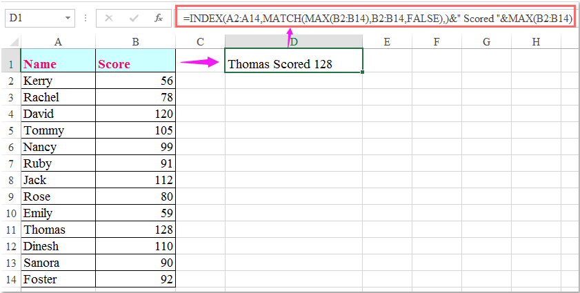
1。名前を表示したい空白セル（例：セル C2）に、次の数式を入力してください。

=INDEX(A2:A14,MATCH(MAX(B2:B14),B2:B14,FALSE))&" Scored "&MAX(B2:B14)

数式を入力したら、Enterキーを押して確定します。この数式は、最高得点を獲得した最初の名前を返します。たとえば、ジョンとアリスの両方が98 点を獲得していた場合でも、この数式ではリスト上で先に出現する名前のみが返されます。

最高得点に対応する名前を表示する数式を入力

注意事項：

1。上記の数式において、A2:A14は名前を取得したい名前のリスト、B2:B14は得点のリストです。範囲がデータと完全に一致していることを必ず確認してください。
2。この数式は最初に一致した名前のみを返します。複数人が最高得点を共有している場合、すべての名前を表示したいこともあるでしょう。そのようなケースには、後述の実用的な解決策をご参照ください。

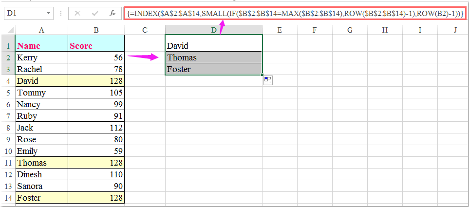
任意のセル（例：D2）に、次の数式を入力してください。

=INDEX($A$2:$A$14,SMALL(IF($B$2:$B$14=MAX($B$2:$B$14),ROW($B$2:$B$14)-1),ROW(B2)-1))

数式を入力したら、Ctrl + Shift + Enterを同時に押してください（Enter キーだけではいけません）。これにより、配列数式が完成し、最高得点を持つ名前が表示されます。その後、そのセルを選択してフィルハンドルを下方向にドラッグします。エラー値が表示されるまでドラッグを続けると、各行に最高得点を共有する別の人物の名前が順に表示されていきます。同点の得点者がいて、すべての優勝者を一覧で確認したい場合に、特に便利です！

最高得点に対応するすべての名前を表示する数式を入力

Excel のバージョンが動的配列（Office 365 やExcel 2021 以降など）に対応している場合は、さらにシンプルなアプローチが可能です。次の数式をセルに入力し（Enter キーを押すだけで OK）、ぜひお試しください。

=FILTER(A2:A14,B2:B14=MAX(B2:B14))

この数式を使えば、トップスコアを獲得したすべての名前が自動的に下のセルにスピル表示されます。ドラッグ操作も特別なキーボードショートカットも不要で、最新版のExcel では非常に便利かつ効果的です。

数式はクイックルックアップに強力ですが、数千行にも及ぶ大規模データセットではパフォーマンスに影響を及ぼすことがあります。また、行の追加や削除が発生した際には、正しい結果を得るため、常に範囲参照を正確に保つ必要があります。そのため、データ選択は必ず再確認してください。

VBA コード – 最高得点に対応する名前を自動的に検索・表示する

VBA マクロを使えば、数式が複雑化したり大規模なリストに対して不十分になった場合でも、データセット内で最高得点を獲得したすべての名前を柔軟かつ自動的に検索・表示できます。VBA ではレポート要件に応じてロジックをカスタマイズでき、更新も自動で処理されるため、繰り返しの分析やバッチ処理に非常に役立ちます。

1。Excel ワークブックを開き、開発タブのVisual Basicをクリックします。Microsoft Visual Basic for Applicationsウィンドウが表示されたら、挿入メニューから標準モジュールをクリックして、空のモジュールを挿入します。

次の VBA コードをモジュールウィンドウにコピー＆ペーストしてください。

Sub ShowTopNames()
    Dim rngNames As Range, rngScores As Range, outCell As Range
    Dim nArr As Variant, sArr As Variant
    Dim i As Long, maxVal As Double, hasVal As Boolean
    Dim namesBuf As String
    On Error Resume Next
    Set rngNames = Application.InputBox("Please select the name column (single column)", "Top Names", Type:=8)
    Set rngScores = Application.InputBox("Please select the score column (single column, same rows as names)", "Top Names", Type:=8)
    Set outCell = Application.InputBox("Please select the output cell (optional, click Cancel to skip)", "Top Names", Type:=8)
    On Error GoTo 0
    If rngNames Is Nothing Or rngScores Is Nothing Then Exit Sub
    If rngNames.Rows.Count <> rngScores.Rows.Count Or rngNames.Columns.Count <> 1 Or rngScores.Columns.Count <> 1 Then
        MsgBox "Range mismatch: Name column and score column must be single columns with the same number of rows.", vbExclamation
        Exit Sub
    End If
    nArr = rngNames.Value2
    sArr = rngScores.Value2
    hasVal = False
    For i = 1 To UBound(sArr, 1)
        If IsNumeric(sArr(i, 1)) And Not IsEmpty(sArr(i, 1)) Then
            If Not hasVal Then
                maxVal = CDbl(sArr(i, 1))
                hasVal = True
            ElseIf CDbl(sArr(i, 1)) > maxVal Then
                maxVal = CDbl(sArr(i, 1))
            End If
        End If
    Next i
    If Not hasVal Then
        MsgBox "No valid numeric values found in the score column.", vbInformation
        Exit Sub
    End If
    rngNames.EntireRow.Interior.ColorIndex = xlNone
    For i = 1 To UBound(sArr, 1)
        If IsNumeric(sArr(i, 1)) Then
            If CDbl(sArr(i, 1)) = maxVal Then
                rngNames.Cells(i, 1).EntireRow.Interior.Color = RGB(255, 255, 153) ' Light yellow
                If Len(namesBuf) > 0 Then namesBuf = namesBuf & ", "
                namesBuf = namesBuf & CStr(nArr(i, 1))
            End If
        End If
    Next i
    If Not outCell Is Nothing Then
        outCell.Value = "Top Score: " & maxVal & " | Name(s): " & namesBuf
    End If
    MsgBox "Top Score = " & maxVal & vbCrLf & "Name(s): " & namesBuf, vbInformation, "Highest Score"
End Sub

2。その後、F5キーを押してこのコードを実行します。以下の3 つのプロンプトが表示されます。名前の列を選択してください（単一列）。名前部分のみをドラッグ選択します（例：A2:A14）→OK。得点の列を選択してください（単一列で、名前と同じ行範囲）。得点をドラッグ選択します（例：B2:B14）→OK。出力先セルを選択してください（任意）。結果を表示したいセル（例：D2）をクリックします。

コードを実行すると、指定したセルに結果が表示され、同点のトップスコアを獲得したすべての行が薄い黄色でハイライトされます。

PivotTable – PivotTable を使用して最高得点に対応する名前を表示する

Excel のピボットテーブルは、データの分析や集計を視覚的かつインタラクティブに行える強力な手段です。大規模なデータセットの処理やグループごとの分析に特に適しており、「各カテゴリ内または全体でのトップスコア」など、特定の最大値を素早く見つけるのにも最適です。数式やコーディングが不要なため、ポイント＆クリック操作を好むユーザーはもちろん、定期的なレポート作成タスクにもぴったりです。

この要件を満たすためのピボットテーブルを使った基本的なワークフローは次のとおりです。

1。データ範囲内（名前と得点の両方の列を含む）の任意のセルを選択し、挿入 > ピボットテーブルをクリックします。ダイアログボックスでデータ範囲を確認し、ピボットテーブルを新規ワークシートまたは既存のワークシートのいずれかに配置するように選択します。

2。ピボットテーブルフィールドウィンドウで、名前フィールドを行ラベルエリアに、得点フィールドを値エリアにドラッグします。値エリアはデフォルトで「合計」または「個数」となっています。得点フィールドのドロップダウン矢印を値エリア内でクリックし、「値の集計方法フィールドの設定」を選択して、要約関数として最大を選び、OKをクリックします。

3。これでピボットテーブルに各名前の最高得点が表示されます。「得点の最大」列を降順で並べ替えると、全体のトップスコアが上位に表示され、その名前が最高（または同率最高）得点者となります。さらに、フィルターや条件付き書式を適用して、視覚的に強調することもできます。

トップスコアの人物（複数可）のみを表示したい場合は、「値のフィルター」を適用しましょう。名前の行ラベルにあるドロップダウン矢印をクリックし、値のフィルター > 次と等しいを選択して、値を最高得点に設定します（一時的にデータを並べ替えたり、「得点の最大」列の最大値を確認したりすれば、簡単に特定できます）。これで、レポートを優勝者の名前に絞り込めます！

ピボットテーブルはデータ探索に最適な強力なツールです。データを簡単に更新・拡張・フィルターでき、ピボットテーブルを更新すれば結果が自動的に再計算されます。ただし、データセットが頻繁に変更される場合は、新しいデータを追加した後、必ずピボットテーブルを右クリックして更新を選択してください。

ピボットテーブルは初期設定に少し時間がかかる場合がありますが、部門やチームなど追加のカテゴリがデータに含まれている場合でも、柔軟なレポート作成やグループ間の比較が可能になります。

集計や並べ替えで問題が発生した場合は、データに空白セルが含まれていないことと、条件名の表記が一貫していることをご確認ください。大規模なリストをご利用の際は、ソース範囲に十分ご注意いただくことで、ピボットテーブルがすべての関連データを正確に反映できるようになります。

KUTOOLS AI でExcel の魔法を解き放ちましょう

スマート実行：セル操作、データ分析、チャート作成をすべてシンプルなコマンドで実現します。
カスタム数式：ワークフローの効率化に役立つ、あなただけのカスタマイズ数式を生成します。
VBA コーディング：VBA コードを簡単に記述・実装できます。
数式の解釈：複雑な数式が簡単に理解できます。
テキスト翻訳：スプレッドシート内で言語の壁を乗り越えましょう！

AI 搭載のツールでExcel の機能をさらに強化しましょう。今すぐダウンロードして、これまでにない効率を体験してください！

最高の Office 業務効率化ツール

🤖	KUTOOLS AI アシスタント：次に基づいてデータ分析を革新します：インテリジェント実行｜コード生成｜カスタム数式作成｜データ分析とチャート生成｜拡張機能呼び出し…
	人気の機能：検索・ハイライト、または重複をマーキング｜空白行を削除する｜データを失うことなく列の結合またはセルを｜数式を使用しない四捨五入...
	スーパー LOOKUP：複数条件 VLookup ｜複数値 VLookup ｜複数シート間 VLookup ｜ファジーマッチ....
	高度なドロップダウンリスト：ドロップダウンリストをすばやく作成｜連動型ドロップダウンリスト｜複数選択可能なドロップダウンリスト....
	列マネージャー：指定した数の列を追加｜列の移動｜非表示列の表示状態を切り替え｜範囲および列の比較...
	注目の機能：グリッドフォーカス｜デザインビュー｜強化された数式バー｜ワークブックとシートマネージャー｜リソースライブラリ（オートテキスト）｜日付ピッカー｜ワークシートの統合｜暗号化／セルの復号化｜リストからメール送信｜スーパーフィルター｜特殊フィルタ（太字のフォントを持つセルをフィルタリング／斜体／取り消し線。。。）。。。
	トップ15 ツールセット：12 テキストツール（テキストの追加、特定の文字を削除、...）｜ 50+チャートタイプ（ガントチャート、...）｜ 40+実用的関数（誕生日に基づいて年齢を計算します、...）｜ 19 挿入ツール（QR コードを挿入、パスから画像を挿入、...）｜ 12 変換ツール（単語に変換する、為替レートの変換、...）｜ 7 結合と分割ツール（高度な行のマージ、セルの分割、...）｜さらに多数

Kutools はお好みの言語でご利用いただけます。英語、スペイン語、ドイツ語、フランス語、中国語、および40+の他の言語をサポートしています！

Kutools for Excel でExcel スキルを強化し、これまでにない効率を体験しましょう。Kutools for Excel は、生産性を高め、時間を大幅に節約できる高度な機能を300 以上提供します。最も必要な機能を今すぐ入手するにはこちらをクリック。。。

Kutools for Excel の詳細はこちら。。。無料ダウンロード。。。

Office Tab は Office にタブインターフェースをもたらし、作業を大幅に簡単にします

Word、Excel、PowerPoint でタブを使った編集と閲覧を有効にします。Publisher、Access、Visio、Project でもご利用いただけます。
複数のドキュメントを、新しいウィンドウではなく、同じウィンドウ内の新しいタブで開いたり作成したりできます。
日々の生産性を50％も向上させ、毎日数百回ものマウスクリックを削減します！

Office Tab の詳細はこちら。。。無料ダウンロード。。。

すべてのKutools アドインが、たった1 つのインストーラーで完結。

Kutools for Officeスイートには、Excel ・Word ・Outlook ・PowerPoint 用のアドインと Office Tab Pro が含まれており、複数の Office アプリを横断して作業するチームに最適です。

オールインワンスイート— Excel、Word、Outlook、PowerPoint 用アドイン＋Office Tab Pro
インストーラー1 つ、ライセンス1 つ— 数分でセットアップ可能（MSI 対応）
連携してさらにパワーアップ— Office アプリ全体で生産性が向上
30 日間のフル機能トライアル— 登録不要、クレジットカード不要
最高のお得感— 個別アドイン購入よりお得

Kutools for Office の詳細はこちら。。。無料ダウンロード。。。