Excel でセルに複数の値のいずれかが含まれているかどうかを確認するには、どうすればよいですか？

著者Xiaoyang変更日2025-07-22

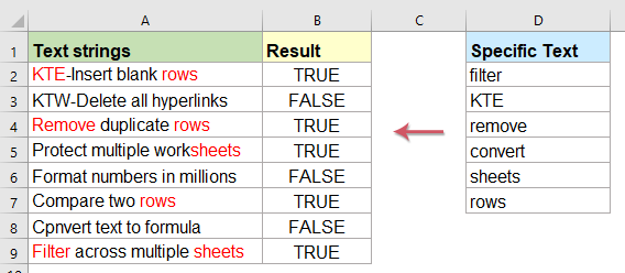
ビジネス、分析、データレビューなどさまざまなシーンで、A 列にテキスト文字列のリストがあり、各セルが特定の値セット（例：D2:D7 の範囲に記載されたもの）のいずれかを含んでいるかどうかを確認したいことがあります。たとえば、アンケート回答、ログデータ、製品リストなどで、各エントリーに特定のキーワード、製品コード、禁止用語が含まれているかを判定することが重要です。そのような場合、セルが指定リストのいずれかの項目を含んでいればExcel にTrueを返させ、含まれていない場合はFalseを返させる必要があります（下のスクリーンショット参照）。本記事では、セルが別範囲内の複数の値のいずれかを含んでいるかをチェックする実用的な方法を解説し、Excel のさまざまなバージョンやユーザーのニーズに応じた複数のアプローチをご紹介します。

数式を使用して、セルにリスト内の複数の値のいずれかが含まれているかを確認する

数式を使用して、セルにリスト内の複数の値のいずれかが含まれている場合、その一致項目を表示する

便利な機能を使用して、セルにリスト内の複数の値のいずれかが含まれている場合、その一致項目をハイライトする

条件付き書式を使用するを使用して、セルに複数の値のいずれかが含まれているかを確認する

数式を使用して、セルにリスト内の複数の値のいずれかが含まれているかを確認する

セルに別の範囲からのテキスト値が含まれているかどうかを判断するには、大規模なデータセットでも効率的に動作する配列数式が活用できます。この方法は、結果を論理値（)True/False）として得たい場合に特に便利です。その論理値は、さらに他の数式やフィルタリング、論理テストにもそのまま利用できます。このテクニックは、最新のほとんどのExcel バージョンでご利用いただけます。

空白セル（例：元のデータの隣にある B2 セル）に次の数式を入力し、必要に応じてフィルハンドルを下にドラッグして他のセルにも適用してください。対象セルに指定された範囲内のテキスト値が含まれている場合は True、そうでない場合は False を返します（スクリーンショット参照）。

=SUMPRODUCT(--ISNUMBER(SEARCH($D$2:$D$7,A2)))>0

数式を使用して、セルが複数の値のいずれかを含んでいるかどうかを確認

ヒントと注意点：

この数式は大文字と小文字を区別しません。大文字と小文字を厳密に区別する必要がある場合は、ヘルパー列をご利用いただくか、より高度な方法で数式を組み合わせることをご検討ください。
True/False の代わりに「はい」または「いいえ」の結果を返すように調整するには、次の数式を使用してください：

=IF(SUMPRODUCT(--ISNUMBER(SEARCH($D$2:$D$6,A2))),「Yes」,「No」)

数式を使用して結果を「はい」または「いいえ」で表示

D2:D7は値の範囲（「リスト」）です。A2はテスト対象のセルです。
SEARCH 関数は有効なテキスト入力を必要とするため、空白セルやテキスト以外のデータにはご注意ください。空白値が含まれている場合、「True」など予期しない結果が返される可能性があります。

数式を使用して、セルにリスト内の複数の値のいずれかが含まれている場合、その一致項目を表示する

単に True/False の結果を表示するだけでなく、リスト内のどの値が各セルに実際に出現しているかを示す方が有益な場合があります。たとえば、製品説明やコメントを特定のキーワードに対してスキャンする際、さらなる分析やレポートのために見つかったすべての値を取得したいことがあります。以下の数式を使えば、一致したすべての値をカンマ区切りで表示できます（図参照）：

セルが複数の値のいずれかを含んでいる場合に一致するものを表示

空白セル（例：B2）にこの数式を入力すると、D2:D7 内のA2に見つかったすべての値がカンマ区切りでリストされます：

=TEXTJOIN(", ", TRUE, IF(COUNTIF(A2, 「*」&$D$2:$D$7&「*」), $D$2:$D$7, 「」))

注記：ここでは、D2:D7が検索対象の値の範囲で、A2が検索するセルです。

Ctrl + Shift + Enterを押して数式を確定したら、結果のスクリーンショットに示されているように、フィルハンドルを下にドラッグして他の行にも数式を適用できます。

セルが複数の値のいずれかを含んでいる場合に一致するものを表示するための数式を適用

TEXTJOIN 関数は、Excel 2019 および Office 365 でのみご利用いただけます。それ以前のバージョンのExcel をご利用の場合には、次の配列数式を空白セルに入力し、Ctrl + Shift + Enterを押してください：

=IFERROR(INDEX($D$2:$D$7, SMALL(IF(COUNTIF($A2, 「*」&$D$2:$D$7&「*」), MATCH(ROW($D$2:$D$7), ROW($D$2:$D$7)), 「」), COLUMNS($F$1:F1))), 「」)

可能な限り多くの列にわたって数式を右方向にドラッグして、すべての一致項目をキャプチャします。一致項目が少ない場合は、余分な列は空白のままになります。この形式は、一致項目を別々の列にリストする必要がある場合に特に役立ちます：

セルが複数の値のいずれかを含んでいる場合に、別々の列で一致するものを表示するための数式を適用

エラーが発生した場合は、まず範囲を再確認し、D2:D7の領域が正しいことをご確認ください。また、お使いのロケールに応じて、正しい区切り文字（カンマまたはセミコロン）を使用しているかも合わせてご確認ください。

便利な機能を使用して、セルにリスト内の複数の値のいずれかが含まれている場合、その一致項目をハイライトする

リスト内の任意の値と一致するキーワードやフレーズを各セル内で視覚的にハイライトしたい場合、重要なデータを目立たせることで、レビューしたりアクションを促したりするのに役立ちます。キーワードのマーキング機能は、Kutools for Excelに搭載されており、数式や VBA コードを記述することなく、データ範囲内の指定された単語のすべてのインスタンスを瞬時にハイライトできます。この機能は特に、大規模なシートや複雑なデータセットで手動チェックが非現実的となるようなシーンに最適です。

Kutools for Excelは300 以上の高度な機能を提供し、複雑な作業を効率化して、創造性と生産性を高めます。AI 機能と統合されたKutools は、正確にタスクを自動化し、データ管理を簡単にします。Kutools for Excel の詳細情報。。。 無料トライアル。。。

Kutools for Excel をインストールした後、次の手順に従ってください：

1。「Kutools 」>「テキスト」>「キーワードのマーキング」の順に選択して、図のようにダイアログ「キーワードのマーキング」を起動します。

Kutools の「キーワードをマーク」機能をクリック

2。キーワードのマーキングダイアログで、次の操作を行います。

対象のデータ範囲を範囲ボックスから選択してください。
キーワードボックスにキーワードを入力するか、カンマ区切りで手動入力してください。
キーワードのフォント色オプションでハイライト色を指定できます。

ダイアログボックスでオプションを設定

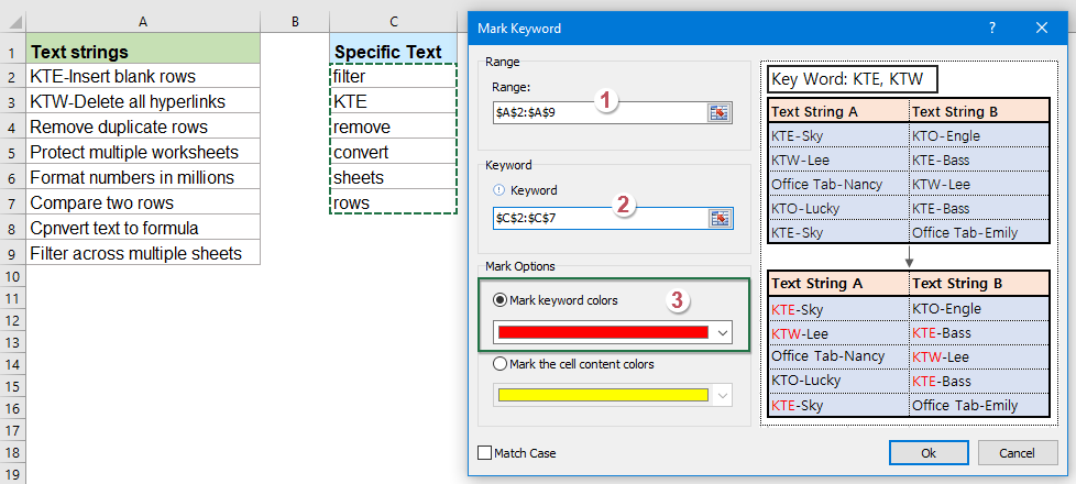
3。OKをクリックすると、一致するすべてのWord が選択範囲内で、指定したフォント色でハイライト表示されます。

すべての一致するテキストがハイライトされました

この機能は、一致したキーワードの表示形式を直接変更するため、数式の出力を理解できないチームメンバーにとっても、結果のレビューまたは共有が直感的になります。
キーワードリストやテキスト範囲が非常に大きい場合、または複数の条件を一度にハイライトする必要がある場合に特に効果的です。
意図しないハイライトを避けるため、確定する前に必ず範囲を選択し、キーワードの入力を再確認してください。

複数の値のいずれかをセルが含むかどうかを条件付き書式を使用するを使って確認する

Excel に標準搭載されている条件付き書式を使用するのも、指定リスト内のいずれかの値を含むセルをハイライト表示するための効果的な方法です。この方法を使えば、データレビュー、エラーチェック、コンプライアンス作業などの際に、関連する行を一目で視覚的に識別できます。Kutools のキーワードのマーキング機能とは異なり、この方法ではアドインを必要としないため、標準のExcel 環境でもすぐにご利用いただけます。

条件付き書式を使用するを数式と共に使用する手順は次のとおりです。

監視対象にするには、データ範囲内のセル（例：A2:A20）を選択してください。
ホームタブに移動し、条件付き書式を使用する＞新規ルールをクリックします。
「新しい書式設定ルール」ダイアログで、数式を使用して書式設定するセルを決定するを選択します。
D2:D7 に値が含まれており、A2 が最初のデータセルであると仮定して、次の数式を入力します：

=SUMPRODUCT(--ISNUMBER(SEARCH($D$2:$D$7,A2)))>0

書式設定をクリックして、希望の書式（例：塗りつぶし色）を指定し、OKを押してください。

D2:D7 リスト内のいずれかの項目を含むすべてのセルが、自動的にハイライト表示されるようになります。

この方法は動的です。範囲 D2:D7 を更新すると、書式設定もそれに応じて自動的に調整されます。
条件付き書式は表示専用の機能です。セルを視覚的にマークするだけで、別の列に結果を出力したり、さらなる計算に利用したりすることはできません。
数式ベースの条件付き書式は強力ですが、データセットが非常に大きい場合には繰り返し計算が発生し、パフォーマンスが低下することがあります。
SEARCH 関数は大文字と小文字を区別しない点にご注意ください。この関数で大文字と小文字を区別するには、より高度なテクニックやヘルパー列が必要になる場合があります。

最高の Office 業務効率化ツール

🤖	KUTOOLS AI アシスタント：次に基づいてデータ分析を革新します：インテリジェント実行｜コード生成｜カスタム数式作成｜データ分析とチャート生成｜拡張機能呼び出し…
	人気の機能：検索・ハイライト、または重複をマーキング｜空白行を削除する｜データを失うことなく列の結合またはセルを｜数式を使用しない四捨五入...
	スーパー LOOKUP：複数条件 VLookup ｜複数値 VLookup ｜複数シート間 VLookup ｜ファジーマッチ....
	高度なドロップダウンリスト：ドロップダウンリストをすばやく作成｜連動型ドロップダウンリスト｜複数選択可能なドロップダウンリスト....
	列マネージャー：指定した数の列を追加｜列の移動｜非表示列の表示状態を切り替え｜範囲および列の比較...
	注目の機能：グリッドフォーカス｜デザインビュー｜強化された数式バー｜ワークブックとシートマネージャー｜リソースライブラリ（オートテキスト）｜日付ピッカー｜ワークシートの統合｜暗号化／セルの復号化｜リストからメール送信｜スーパーフィルター｜特殊フィルタ（太字のフォントを持つセルをフィルタリング／斜体／取り消し線。。。）。。。
	トップ15 ツールセット：12 テキストツール（テキストの追加、特定の文字を削除、...）｜ 50+チャートタイプ（ガントチャート、...）｜ 40+実用的関数（誕生日に基づいて年齢を計算します、...）｜ 19 挿入ツール（QR コードを挿入、パスから画像を挿入、...）｜ 12 変換ツール（単語に変換する、為替レートの変換、...）｜ 7 結合と分割ツール（高度な行のマージ、セルの分割、...）｜さらに多数

Kutools はお好みの言語でご利用いただけます。英語、スペイン語、ドイツ語、フランス語、中国語、および40+の他の言語をサポートしています！

Kutools for Excel でExcel スキルを強化し、これまでにない効率を体験しましょう。Kutools for Excel は、生産性を高め、時間を大幅に節約できる高度な機能を300 以上提供します。最も必要な機能を今すぐ入手するにはこちらをクリック。。。

Kutools for Excel の詳細はこちら。。。無料ダウンロード。。。

Office Tab は Office にタブインターフェースをもたらし、作業を大幅に簡単にします

Word、Excel、PowerPoint でタブを使った編集と閲覧を有効にします。Publisher、Access、Visio、Project でもご利用いただけます。
複数のドキュメントを、新しいウィンドウではなく、同じウィンドウ内の新しいタブで開いたり作成したりできます。
日々の生産性を50％も向上させ、毎日数百回ものマウスクリックを削減します！