ドロップダウンリストの先頭に空白ではなく、最初の項目を表示するにはどうすればよいですか？

著者Xiaoyang変更日2025-07-15

Excel ワークシートのドロップダウンリストは、データ入力を効率化・標準化するための実用的な機能です。ユーザーは個別に入力する代わりに、事前に定義された選択肢から簡単に選べます。しかし、ドロップダウンセルをクリックした際に、最初の選択肢が実際のデータ項目ではなく空白として表示されることがあります。この問題は、ソースデータリストを編集した後に末尾に空白行が残っていたり、末尾近くの項目を削除した結果、データ検証がリストの先頭に意図しない空のスロットを含んでしまう場合によく発生します。特に長いリストでは、毎回空白エントリをスキップして最初の有効な項目までスクロールしなければならず、非効率でイライラすることがあります。

ドロップダウンリストの先頭項目が空白になっているスクリーンショット

この問題に対処すれば、ユーザーの利便性が高まるだけでなく、誤って空白値を選択してしまうリスクも軽減され、その後のデータ処理やレポート作成に悪影響が及ぶのを防げます。本記事では、ドロップダウンリストの先頭に常に最初の項目を表示し、不要な空白を確実に排除するための実践的な方法をご紹介します。

データ検証機能でドロップダウンリストの先頭に最初の項目を表示する

VBA コードでドロップダウンリストの先頭に自動的に最初の項目を表示する

Excel テーブルをソース範囲として使用する

データ検証機能でドロップダウンリストの先頭に最初の項目を表示する

ドロップダウンリストの先頭に空白エントリが表示されないようにする効果的な方法の一つは、正しい範囲を動的に判定する数式を使ってデータ検証を設定することです。このアプローチにより、データ削除によって空行が生じても、ソースリスト内で実際にデータが入力されているセルだけがリストに含まれるようになります。この解決策は、ソースリストを頻繁に変更するユーザーや、マクロを使わずシンプルな数式ベースの調整を好むユーザーに特に適しています。

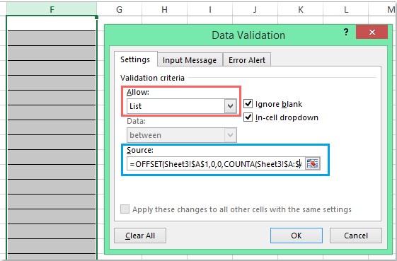
1。ドロップダウンリストを作成したいセルを選択し、Excel のリボンからデータタブのデータの入力規則をクリックします。データの入力規則ダイアログボックスが下図のように開きます。

データ検証ドロップダウンリストを挿入しているスクリーンショット

2。「データの入力規則」ダイアログの設定タブで、許可をリストに設定します。元ボックスに、実際のデータが含まれる範囲を動的に参照する次の数式を入力します。

=OFFSET(Sheet3!$A$1,0,0,COUNTA(Sheet3!$A:$A)-1,1)

注：この数式では、Sheet3はソースデータが存在するシートを、A1はリストの開始セルをそれぞれ指します。ワークシートのレイアウトに応じて、必要に応じて調整してください。COUNTA 関数を使用すると、A1 以降の空白でないセルのみが対象となります。ただし、ソースリスト内に（末尾以外の場所に）意図的に空白行が含まれている場合、この方法ではそれらが完全に除外されない可能性があるため、最良の結果を得るにはソースリストを連続した範囲で保つようにしてください。

数式を使用してデータ検証設定を構成しているスクリーンショット

3。設定を適用するには、OKをクリックします。これにより、設定したドロップダウンリストのセルをクリックすると、リストの先頭に最初の実際のデータ項目が表示されるようになります。この状態は、ソースデータが変更されても、列 A のすべての項目が範囲に含まれており、かつデータの主要ブロック内に空白セルがない限り維持されます。下図にその結果を示します。

リストの先頭に最初の項目が表示された最終的なドロップダウンリストを示すスクリーンショット

ヒント：後でソースリストを拡張または縮小する必要があっても、データ検証の設定を更新する必要はありません。範囲の先頭に空白セルがなければ、数式は自動的に調整されます。ただし、リスト内（末尾以外）に空白セルがある場合、計算ではスキップされますが、ドロップダウンに意図しないギャップが生じる可能性がありますのでご注意ください。

潜在的な問題：ソース範囲に意図的なギャップが含まれる可能性がある場合や、結合セル・非連続データが存在する場合は、Excel テーブルをソース範囲として使用するか、以下に示す VBA メソッドをご検討ください。より柔軟に対応できます。

VBA コードでドロップダウンリストの先頭に自動的に最初の項目を表示する

状況によっては、データ検証の元を調整するだけでは不十分な場合があります。たとえば、データが頻繁に更新されるケースや、ソース範囲の構造上、空白が生じるリスクがある場合などが該当します。簡単な VBA コードを活用すれば、データ検証が設定されたセルがアクティブになった瞬間、ドロップダウンリストの最初の有効な項目が自動的に選択・表示されるようにできます。これにより、ユーザーのクリック操作を最小限に抑え、データ入力のスピードも向上します。

素晴らしい！Excel でChrome、Edge、Firefox、Safari のような効率的な Tabs をご利用いただけます！
毎日数千回のマウスクリックを削減し、50% もの時間を節約できます！

1。ドロップダウンリストを挿入した後、そのドロップダウンを含むシートタブを右クリックし、コンテキストメニューからコードの表示を選択してください。「Microsoft Visual Basic for Applications」エディターが起動します。ウィンドウ内に表示される該当するワークシートモジュール（標準モジュールではない）に、次のコードを貼り付けてください。このコードはバックグラウンドで動作し、検証セルを選択するたびにドロップダウンを自動的にリセットします。

VBA コード：ドロップダウンリストで最初のデータ項目を自動的に表示する：

Private Sub Worksheet_SelectionChange(ByVal Target As Range)
'Updateby Extendoffice 20160725
    Dim xFormula As String
    On Error GoTo Out:
    xFormula = Target.Cells(1).Validation.Formula1
    If Left(xFormula, 1) = "=" Then
        Target.Cells(1) = Range(Mid(xFormula, 1)).Cells(1).Value
    End If
Out:
End Sub

VBAコードの使用方法を示すスクリーンショット

2。コードを貼り付けたら、ブックを保存してください（マクロを有効にするため、.xlsm 拡張子のファイルとして保存することをおすすめします）。その後、VBA エディターを閉じてシートに戻り、ドロップダウンリストが設定されたセルをクリックしてみましょう。セルがアクティブになると、ドロップダウンの最初の項目が自動的に表示されます。

ヒントと留意点：この VBA アプローチは、ユーザーにシームレスな体験を提供したい場合に最適です。特に、動的または長いソースリスト、あるいは避けられない空白エントリを含むリストでその真価を発揮します。ただし、この機能を有効にするにはマクロを有効化する必要があるため、セキュリティ上の理由でマクロの使用が制限されている環境では、他のユーザーに事前に知らせておくことをお勧めします。

トラブルシューティング：コードが正しく動作しない場合は、VBA エディターで対象のワークシートコードウィンドウに正しく配置されているか、再度ご確認ください。また、ドロップダウンリストが標準的なデータ検証リストを使用しているかも併せてご確認ください。

制限事項：この VBA ソリューションは、ユーザーがドロップダウン付きのセルを選択した場合にのみ動作します。数式の計算結果や貼り付けなど、他の方法でセルに値が入力された場合には反応しません。また、セルからドロップダウンを削除したり、VBA コードが含まれない別のシートにセルを移動したりすると、自動選択機能は失われます。

Excel テーブルをソース範囲として使用する

ドロップダウンのソースリストが動的で、より高い保守性が求められる場合は、ソースリストをExcel テーブルに変換することをご検討ください。テーブルはデータの追加や削除に応じて自動的にサイズを調整するため、リストを常に最新の状態に保つことができます。ただし、Excel テーブルは空白セルを自動的には除外しません。テーブル内に空白エントリが含まれる場合、それらはドロップダウンリストにもそのまま表示されます（Excel 365 およびExcel 2021 で利用可能な FILTER 関数などを用いて明示的に除外しない限り）。

1。ソースデータを選択してCtrl + Tを押し、テーブルに変換します。先頭に空白がないことを確認し、「テーブルのデザイン」タブからテーブルにMyListなどわかりやすい名前を付けましょう。

2。データ検証を設定する際は、テーブルの列に対して構造化参照を使用します。「データの入力規則」の元に、次のように入力してください。

=INDIRECT("MyList[Column1]")

Column1を実際の列名（列見出し）に置き換えてください。これにより、テーブルの該当列に入力済みのすべての項目が自動的に反映され、データを更新してもリストの整合性が常に保たれます。

このアプローチは、ソースデータが定期的に更新され、複数のユーザーが検証リストを効率よく管理する必要がある環境に特に適しています。

最高の Office 業務効率化ツール

🤖	KUTOOLS AI アシスタント：次に基づいてデータ分析を革新します：インテリジェント実行｜コード生成｜カスタム数式作成｜データ分析とチャート生成｜拡張機能呼び出し…
	人気の機能：検索・ハイライト、または重複をマーキング｜空白行を削除する｜データを失うことなく列の結合またはセルを｜数式を使用しない四捨五入...
	スーパー LOOKUP：複数条件 VLookup ｜複数値 VLookup ｜複数シート間 VLookup ｜ファジーマッチ....
	高度なドロップダウンリスト：ドロップダウンリストをすばやく作成｜連動型ドロップダウンリスト｜複数選択可能なドロップダウンリスト....
	列マネージャー：指定した数の列を追加｜列の移動｜非表示列の表示状態を切り替え｜範囲および列の比較...
	注目の機能：グリッドフォーカス｜デザインビュー｜強化された数式バー｜ワークブックとシートマネージャー｜リソースライブラリ（オートテキスト）｜日付ピッカー｜ワークシートの統合｜暗号化／セルの復号化｜リストからメール送信｜スーパーフィルター｜特殊フィルタ（太字のフォントを持つセルをフィルタリング／斜体／取り消し線。。。）。。。
	トップ15 ツールセット：12 テキストツール（テキストの追加、特定の文字を削除、...）｜ 50+チャートタイプ（ガントチャート、...）｜ 40+実用的関数（誕生日に基づいて年齢を計算します、...）｜ 19 挿入ツール（QR コードを挿入、パスから画像を挿入、...）｜ 12 変換ツール（単語に変換する、為替レートの変換、...）｜ 7 結合と分割ツール（高度な行のマージ、セルの分割、...）｜さらに多数

Kutools はお好みの言語でご利用いただけます。英語、スペイン語、ドイツ語、フランス語、中国語、および40+の他の言語をサポートしています！

Kutools for Excel でExcel スキルを強化し、これまでにない効率を体験しましょう。Kutools for Excel は、生産性を高め、時間を大幅に節約できる高度な機能を300 以上提供します。最も必要な機能を今すぐ入手するにはこちらをクリック。。。

Kutools for Excel の詳細はこちら。。。無料ダウンロード。。。

Office Tab は Office にタブインターフェースをもたらし、作業を大幅に簡単にします

Word、Excel、PowerPoint でタブを使った編集と閲覧を有効にします。Publisher、Access、Visio、Project でもご利用いただけます。
複数のドキュメントを、新しいウィンドウではなく、同じウィンドウ内の新しいタブで開いたり作成したりできます。
日々の生産性を50％も向上させ、毎日数百回ものマウスクリックを削減します！

Office Tab の詳細はこちら。。。無料ダウンロード。。。

すべてのKutools アドインが、たった1 つのインストーラーで完結。

Kutools for Officeスイートには、Excel ・Word ・Outlook ・PowerPoint 用のアドインと Office Tab Pro が含まれており、複数の Office アプリを横断して作業するチームに最適です。

オールインワンスイート— Excel、Word、Outlook、PowerPoint 用アドイン＋Office Tab Pro
インストーラー1 つ、ライセンス1 つ— 数分でセットアップ可能（MSI 対応）
連携してさらにパワーアップ— Office アプリ全体で生産性が向上
30 日間のフル機能トライアル— 登録不要、クレジットカード不要
最高のお得感— 個別アドイン購入よりお得

Kutools for Office の詳細はこちら。。。無料ダウンロード。。。