Excelで値のすべての一致するインスタンスを一覧表示する方法
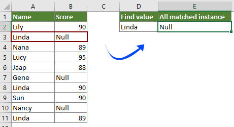
左のスクリーンショットに示されているように、テーブル内の値「Linda」のすべての一致するインスタンスを見つけて一覧表示する必要があります。どのように達成するのでしょうか?この記事の方法を試してみてください。
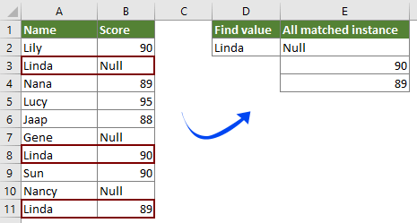
配列数式を使用して値のすべての一致するインスタンスを一覧表示する
Kutools for Excelを使用して値の最初の一致するインスタンスのみを簡単に一覧表示する
VLOOKUPの詳細なチュートリアル...
配列数式を使用して値のすべての一致するインスタンスを一覧表示する
以下の配列数式を使用すると、Excelの特定のテーブル内で値のすべての一致するインスタンスを簡単に一覧表示できます。以下の手順に従ってください。
1. 最初の一致するインスタンスを出力するために空白のセルを選択し、次の数式を入力して、Ctrl + Shift + Enterキーを同時に押します。
=INDEX($B$2:$B$11, SMALL(IF($D$2=$A$2:$A$11, ROW($A$2:$A$11)-ROW($A$2)+1), ROW(1:1)))
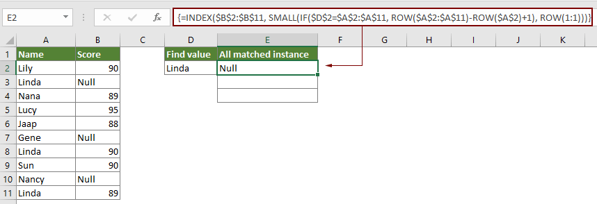
注釈: この数式では、B2:B11は一致するインスタンスが位置する範囲です。A2:A11はすべてのインスタンスを一覧表示する特定の値を含む範囲です。そしてD2には特定の値が含まれています。
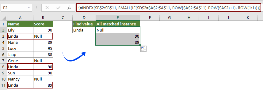
2. 結果セルを選択したままにして、フィルハンドルを下にドラッグして他の一致するインスタンスを取得します。
Kutools for Excelを使用して値の最初の一致するインスタンスのみを簡単に一覧表示する
Kutools for Excelの範囲内でデータを検索する機能を使用すると、数式を覚えることなく、値の最初の一致するインスタンスを簡単に見つけて一覧表示できます。以下の手順に従ってください。
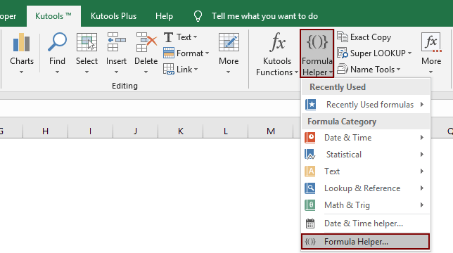
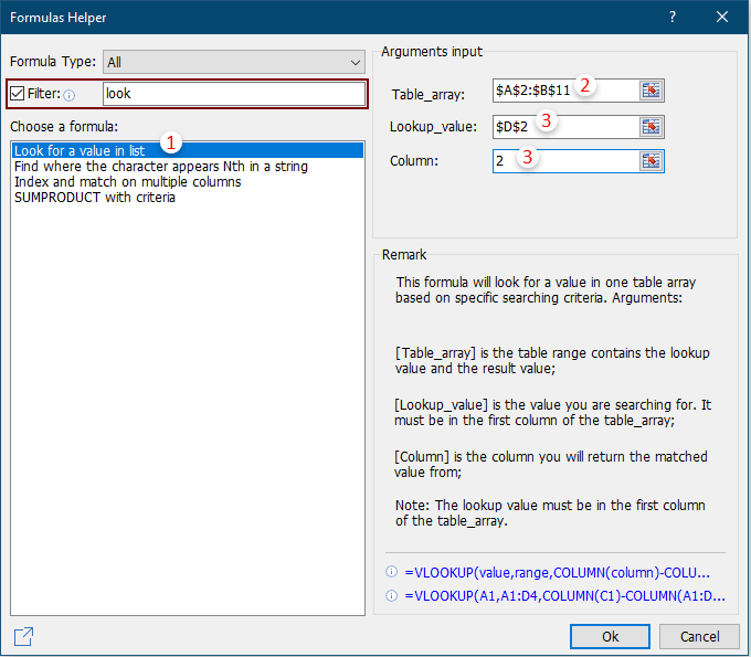
1. 最初の一致するインスタンスを配置する空白のセルを選択し、Kutools > 関数ヘルパー > 関数ヘルパーをクリックします。
2. 関数ヘルパーダイアログボックスで、次の操作を行います。
ヒント: あなたは フィルター ボックスをチェックし、キーワードをテキストボックスに入力して必要な数式をすばやくフィルターできます。
ヒント: 列番号は選択した列数に基づいています。4列を選択し、これが3番目の列の場合、 列 ボックスに番号3を入力する必要があります。
次に、指定された値の最初の一致するインスタンスが以下のスクリーンショットに示されるように一覧表示されます。
このユーティリティを無料で試用したい場合(30日間)、こちらをクリックしてダウンロードし、上記の手順に従って操作を適用してください。
関連する記事
複数のワークシートにわたる値をVLOOKUPで検索する
ワークシートのテーブルで一致する値を返すためにvlookup関数を適用できます。ただし、複数のワークシートにわたって値をvlookupする必要がある場合、どうすればよいでしょうか?この記事では、問題を簡単に解決するための詳細な手順を提供します。
複数の列で一致する値をVLOOKUPで検索して返す
通常、VLOOKUP関数を適用すると、1つの列からのみ一致する値を返すことができます。時には、基準に基づいて複数の列から一致する値を抽出する必要があるかもしれません。ここにその解決策があります。
1つのセルに複数の値をVLOOKUPで返す
通常、VLOOKUP関数を適用すると、基準に一致する複数の値がある場合、最初の1つの結果しか得られません。すべての一致する結果を返し、それらを1つのセルにすべて表示したい場合、どのように達成できますか?
一致する値の行全体をVLOOKUPで検索して返す
通常、vlookup関数を使用すると、同じ行の特定の列からのみ結果を返すことができます。この記事では、特定の基準に基づいてデータの行全体を返す方法を紹介します。
逆方向または逆順でのVLOOKUP
一般的に、VLOOKUP関数は配列テーブル内で左から右に値を検索し、検索値は目標値の左側にある必要があります。しかし、時には目標値を知っていて、逆に検索値を見つけたい場合があります。そのため、Excelで逆方向にvlookupする必要があります。この記事では、この問題を簡単に解決するためのいくつかの方法を紹介します!
最高のオフィス業務効率化ツール
| 🤖 | Kutools AI Aide:データ分析を革新します。主な機能:Intelligent Execution|コード生成|カスタム数式の作成|データの分析とグラフの生成|Kutools Functionsの呼び出し…… |
| 人気の機能:重複の検索・ハイライト・重複をマーキング|空白行を削除|データを失わずに列またはセルを統合|丸める…… | |
| スーパーLOOKUP:複数条件でのVLookup|複数値でのVLookup|複数シートの検索|ファジーマッチ…… | |
| 高度なドロップダウンリスト:ドロップダウンリストを素早く作成|連動ドロップダウンリスト|複数選択ドロップダウンリスト…… | |
| 列マネージャー:指定した数の列を追加 |列の移動 |非表示列の表示/非表示の切替| 範囲&列の比較…… | |
| 注目の機能:グリッドフォーカス|デザインビュー|強化された数式バー|ワークブック&ワークシートの管理|オートテキスト ライブラリ|日付ピッカー|データの統合 |セルの暗号化/復号化|リストで電子メールを送信|スーパーフィルター|特殊フィルタ(太字/斜体/取り消し線などをフィルター)…… | |
| トップ15ツールセット:12 種類のテキストツール(テキストの追加、特定の文字を削除など)|50種類以上のグラフ(ガントチャートなど)|40種類以上の便利な数式(誕生日に基づいて年齢を計算するなど)|19 種類の挿入ツール(QRコードの挿入、パスから画像の挿入など)|12 種類の変換ツール(単語に変換する、通貨変換など)|7種の統合&分割ツール(高度な行のマージ、セルの分割など)|… その他多数 |
Kutools for ExcelでExcelスキルを強化し、これまでにない効率を体感しましょう。 Kutools for Excelは300以上の高度な機能で生産性向上と保存時間を実現します。最も必要な機能はこちらをクリック...
Office TabでOfficeにタブインターフェースを追加し、作業をもっと簡単に
- Word、Excel、PowerPointでタブによる編集・閲覧を実現。
- 新しいウィンドウを開かず、同じウィンドウの新しいタブで複数のドキュメントを開いたり作成できます。
- 生産性が50%向上し、毎日のマウスクリック数を何百回も削減!
全てのKutoolsアドインを一つのインストーラーで
Kutools for Officeスイートは、Excel、Word、Outlook、PowerPoint用アドインとOffice Tab Proをまとめて提供。Officeアプリを横断して働くチームに最適です。
- オールインワンスイート — Excel、Word、Outlook、PowerPoint用アドインとOffice Tab Proが含まれます
- 1つのインストーラー・1つのライセンス —— 数分でセットアップ完了(MSI対応)
- 一括管理でより効率的 —— Officeアプリ間で快適な生産性を発揮
- 30日間フル機能お試し —— 登録やクレジットカード不要
- コストパフォーマンス最適 —— 個別購入よりお得