Excel でチェックボックスを使ってセルや行をハイライト表示するには、どうすればよいでしょうか?
以下のスクリーンショットのように、チェックボックスを使って行やセルをハイライト表示したい場合、チェックボックスをオンにすると指定された行またはセルが自動的にハイライトされるように設定する必要があります。しかし、Excel でこれを実現するにはどうすればよいでしょうか?この記事では、その方法を2 つご紹介します。

チェックボックスを使用してセルまたは行をハイライト表示(条件付き書式を使用する)
VBA コードを使用してチェックボックスでセルまたは行をハイライト表示
条件付き書式を使用するを使用してチェックボックスでセルまたは行をハイライト表示
Excel でチェックボックスを使ってセルや行をハイライト表示するには、条件付き書式のルールを作成できます。以下の手順に従ってください。
ステップ1:すべてのチェックボックスを指定されたセルにリンクする
1。チェックボックス(フォームコントロール)をクリックすると、開発>挿入>チェックボックス(フォームコントロール)からセルごとに1 つずつ手動で挿入する必要があります。
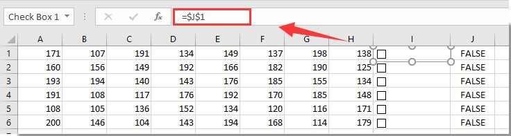
2。これで、列 I のセルにチェックボックスが挿入されました。Enterキーを押す前に、I1 にある最初のチェックボックスを右クリックし、数式バーに数式 =$J1を入力してください。
ヒント:チェックボックスの隣接セルに関連付けられた値を表示したくない場合は、チェックボックスを別のワークシートのセル(例:=Sheet3!$E$1)にリンクできます。
3。すべてのチェックボックスが隣接セルまたは別のワークシートのセルにリンクされるまで、手順1 を繰り返します。
注:すべてのリンクされたセルは連続しており、同じ列内に配置されている必要があります。
ステップ2:条件付き書式を使用するルールを作成する
次に、以下の手順に従って、条件付き書式のルールを作成する必要があります。
1。ハイライト表示したい行をチェックボックスで選択し、ホームタブの条件付き書式を使用する>新しいルールをクリックします。スクリーンショットを参照してください:

2。新しい書式設定ルールダイアログボックスで、以下の操作を行ってください。
2.1 数式を使用して書式設定するセルを決定するを、ルールの種類の選択ボックスで選択します。
2.2 数式 =IF($J1=TRUE,TRUE,FALSE)を「この数式が真である場合に値を書式設定する」ボックスに入力します。
または、チェックボックスが別のワークシートにリンクされている場合は=IF(Sheet3!$E1=TRUE,TRUE,FALSE)を入力します。
2.3 書式設定ボタンをクリックして、行のハイライト表示色を設定します。
2.4 OKボタンをクリックしてください。スクリーンショットを以下に示します:

注: 数式内の$J1または$E1は、チェックボックスの最初のリンクされたセルです。セル参照が列の絶対参照に変更されていることを確認してください()J1 > $J1またはE1 > $E1)。
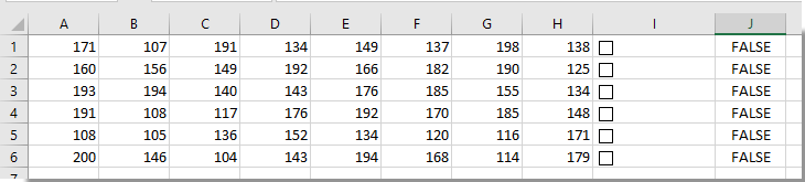
これで条件付き書式のルールが作成されました。チェックボックスをオンにすると、対応する行が以下のスクリーンショットのように自動的にハイライトされます。

VBA コードを使用してチェックボックスでセルまたは行をハイライト表示
次の VBA コードを使えば、Excel でチェックボックスを使ってセルや行をハイライト表示できます。以下の手順に従ってください。
1。チェックボックスでセルまたは行をハイライト表示したいワークシートで、シートタブを右クリックし、コンテキストメニューからコードの表示を選択して、Microsoft Visual Basic for Applicationsウィンドウを開きます。
2。次に、以下の VBA コードをコードウィンドウにコピー&ペーストしてください。
VBA コード:Excel でチェックボックスを使用して行をハイライト表示
Sub AddCheckBox()
Dim xCell As Range
Dim xRng As Range
Dim I As Integer
Dim xChk As CheckBox
On Error Resume Next
InputC:
    Set xRng = Application.InputBox("Please select the column range to insert checkboxes:", "Kutools for Excel", Selection.Address, , , , , 8)
If xRng Is Nothing Then Exit Sub
If xRng.Columns.Count > 1 Then
    MsgBox "The selected range should be a single column", vbInformation, "Kutools fro Excel"
    GoTo InputC
Else
    If xRng.Columns.Count = 1 Then
        For Each xCell In xRng
            With ActiveSheet.CheckBoxes.Add(xCell.Left, _
               xCell.Top, xCell.Width = 15, xCell.Height = 12)
               .LinkedCell = xCell.Offset(, 1).Address(External:=False)
               .Interior.ColorIndex = xlNone
               .Caption = ""
               .Name = "Check Box " & xCell.Row
            End With
            xRng.Rows(xCell.Row).Interior.ColorIndex = xlNone
        Next
    End If
    With xRng
     .Rows.RowHeight = 16
    End With
    xRng.ColumnWidth = 5#
    xRng.Cells(1, 1).Offset(0, 1).Select
    For Each xChk In ActiveSheet.CheckBoxes
      xChk.OnAction = ActiveSheet.Name + ".InsertBgColor"
    Next
End If
End Sub

Sub InsertBgColor()
Dim xName As Integer
Dim xChk As CheckBox
For Each xChk In ActiveSheet.CheckBoxes
  xName = Right(xChk.Name, Len(xChk.Name) - 10)
  If (xName = Range(xChk.LinkedCell).Row) Then
   If (Range(xChk.LinkedCell) = "True") Then
    Range("A" & xName, Range(xChk.LinkedCell).Offset(0, -2)).Interior.ColorIndex = 6
   Else
    Range("A" & xName, Range(xChk.LinkedCell).Offset(0, -2)).Interior.ColorIndex = xlNone
   End If
  End If
Next
End Sub
3。F5キーを押してコードを実行します。()注:F5 キーを適用するには、コードの先頭にカーソルを置く必要があります。)表示されるKutools for Excelダイアログボックスで、チェックボックスを挿入したい範囲を選択し、OKボタンをクリックします。ここでは、範囲として I1:I6 を選択しています。スクリーンショットを参照してください:

4。その後、選択したセルにチェックボックスが挿入されます。いずれかのチェックボックスをオンにすると、対応する行が以下のスクリーンショットのように自動的にハイライト表示されます。

関連記事:
- Excel でチェックボックスをオンにした際に、指定されたセルの値や色を自動的に変更するにはどうすればよいですか?
- Excel でチェックボックスをオンにしたときにセルに日付スタンプを挿入するには、どうすればよいですか?
- Excel でセルの値に基づいてチェックボックスを自動的にオンにするには、どうすればよいですか?
- Excel でチェックボックスに基づいてデータをフィルターするには、どうすればよいでしょうか?
- Excel で行を非表示にした際に、その行にあるチェックボックスも一緒に非表示にするにはどうすればよいですか?
- Excel でチェックボックスを複数含んだドロップダウンリストを作成するには、どうすればよいでしょうか?
最高の Office 業務効率化ツール
| 🤖 | KUTOOLS AI アシスタント:次に基づいてデータ分析を革新します:インテリジェント実行 | コード生成| カスタム数式作成 | データ分析とチャート生成| 拡張機能呼び出し… |
| 人気の機能:検索・ハイライト、または重複をマーキング | 空白行を削除する | データを失うことなく列の結合またはセルを | 数式を使用しない四捨五入... | |
| スーパー LOOKUP:複数条件 VLookup | 複数値 VLookup | 複数シート間 VLookup | ファジーマッチ.... | |
| 高度なドロップダウンリスト:ドロップダウンリストをすばやく作成 | 連動型ドロップダウンリスト | 複数選択可能なドロップダウンリスト.... | |
| 列マネージャー:指定した数の列を追加|列の移動|非表示列の表示状態を切り替え|範囲および列の比較... | |
| 注目の機能:グリッドフォーカス | デザインビュー |強化された数式バー | ワークブックとシートマネージャー | リソースライブラリ(オートテキスト)| 日付ピッカー | ワークシートの統合 | 暗号化/セルの復号化 | リストからメール送信 | スーパーフィルター | 特殊フィルタ(太字のフォントを持つセルをフィルタリング/斜体/取り消し線。。。) 。。。 | |
| トップ15 ツールセット:12 テキストツール(テキストの追加、特定の文字を削除、...)| 50+チャートタイプ(ガントチャート、...)| 40+実用的関数(誕生日に基づいて年齢を計算します、...)| 19 挿入ツール(QR コードを挿入、パスから画像を挿入、...)| 12 変換ツール(単語に変換する、為替レートの変換、...)| 7 結合と分割ツール(高度な行のマージ、セルの分割、...)|さらに多数 |
Kutools for Excel でExcel スキルを強化し、これまでにない効率を体験しましょう。Kutools for Excel は、生産性を高め、時間を大幅に節約できる高度な機能を300 以上提供します。最も必要な機能を今すぐ入手するにはこちらをクリック。。。
Office Tab は Office にタブインターフェースをもたらし、作業を大幅に簡単にします
- Word、Excel、PowerPoint でタブを使った編集と閲覧を有効にします。Publisher、Access、Visio、Project でもご利用いただけます。
- 複数のドキュメントを、新しいウィンドウではなく、同じウィンドウ内の新しいタブで開いたり作成したりできます。
- 日々の生産性を50%も向上させ、毎日数百回ものマウスクリックを削減します!
すべてのKutools アドインが、たった1 つのインストーラーで完結。
Kutools for Officeスイートには、Excel ・Word ・Outlook ・PowerPoint 用のアドインと Office Tab Pro が含まれており、複数の Office アプリを横断して作業するチームに最適です。
- オールインワンスイート— Excel、Word、Outlook、PowerPoint 用アドイン+Office Tab Pro
- インストーラー1 つ、ライセンス1 つ— 数分でセットアップ可能(MSI 対応)
- 連携してさらにパワーアップ— Office アプリ全体で生産性が向上
- 30 日間のフル機能トライアル— 登録不要、クレジットカード不要
- 最高のお得感— 個別アドイン購入よりお得