セルの値に基づいてExcelのセルに画像を動的に挿入するにはどうすればよいですか?
Excelでは、セルの値に基づいて画像を動的に表示する必要がある状況に遭遇することがあります。例えば、特定の名前をセルに入力すると、対応する画像が別のセルに自動的に更新されます。このガイドでは、それを実現するためのステップバイステップの手順を提供します。
セルに入力した値に基づいて画像を動的に挿入および変更する
Kutools for Excelを使用してセルの値に基づいて画像を動的に変更する
セルに入力した値に基づいて画像を動的に挿入および変更する
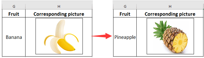
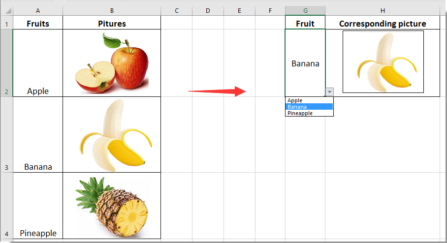
下のスクリーンショットに示すように、G2セルに入力した値に基づいて対応する画像を動的に表示したいとします。G2セルに「バナナ」と入力すると、H2セルにバナナの画像が表示されます。一方、G2セルに「パイナップル」と入力すると、H2セルの画像は対応するパイナップルの画像に変わります。
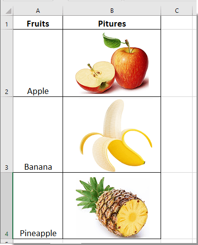
1. ワークシートに2つの列を作成し、最初の列範囲A2:A4には画像の名前を、2番目の列範囲 B2:B4には対応する画像を入れます。スクリーンショットをご覧ください。
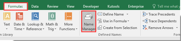
2. 数式 > 名前 をクリックしてください。
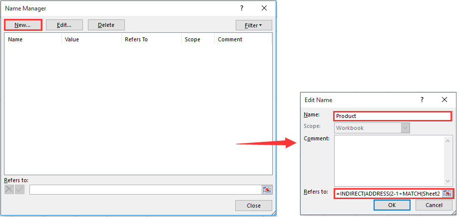
3. 名前の管理ダイアログボックスで、新規ボタンをクリックします。次に名前の編集ダイアログがポップアップするので、名前ボックスに「Product 」を入力し、以下の数式を参照先ボックスに入力してからOKボタンをクリックします。スクリーンショットをご覧ください:
=INDIRECT(ADDRESS(2-1+MATCH(Sheet2!$G$2, Sheet2!$A$2:$A$4, 0), 2))
注釈:
上記の数式の中で必要に応じてこれらを変更できます。
4. 名前の管理ダイアログボックスを閉じます。
5. 画像列から画像を選択し、Ctrl + Cキーを同時に押してコピーします。その後、現在のワークシート内の新しい場所に貼り付けます。ここでは、リンゴの画像をコピーしてH2セルに配置します。

6. G2セルに「Apple」などの果物の名前を入力し、貼り付けた画像をクリックして選択し、数式バーに 「=Product」と入力してEnterキーを押します。スクリーンショットをご覧ください:

これで、G2セルの果物の名前を変更すると、H2セルの画像が対応するものに動的に変わります。
下のスクリーンショットに示すように、G2セルにすべての果物の名前を含むドロップダウンリストを作成することで、果物の名前を迅速に選択できます。
Kutools for Excelを使用してセルの値に基づいて画像を動的に変更する
多くのExcel初心者にとって、上記の方法は扱いにくいものです。そこで、 Kutools for Excelの「画像付きドロップダウンリスト」機能をお勧めします。この機能を使用すると、値と画像が完全に一致する動的なドロップダウンリストを簡単に作成できます。
以下のように、Excelで動的な画像付きドロップダウンリストを作成するために、Kutools for Excelの「画像付きドロップダウンリスト」機能を適用してください。
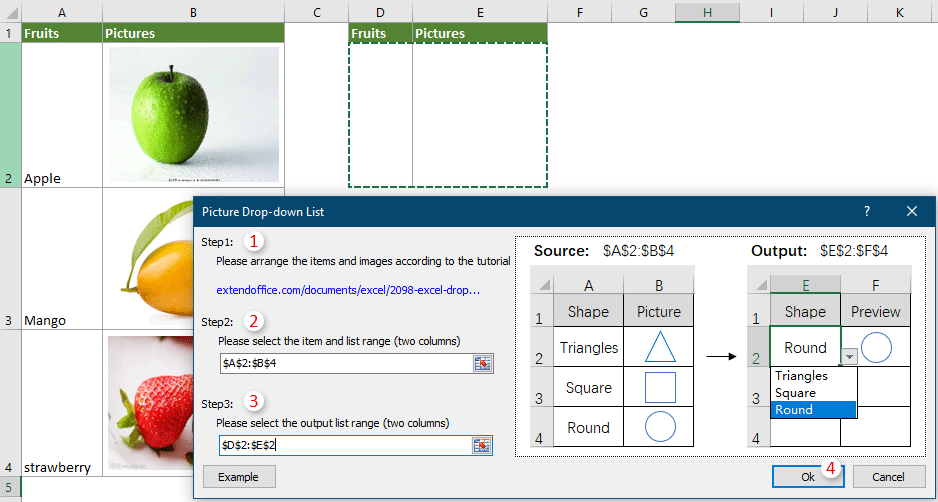
1. まず、下のスクリーンショットに示すように、値とそれに対応する画像を含む2つの列を別々に作成する必要があります。

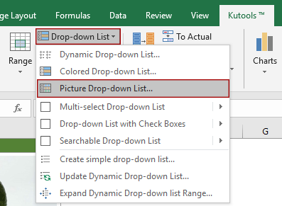
2. Kutools > ドロップダウンリスト > 画像付きドロップダウンリストをクリックします。
3. 「画像付きドロップダウンリスト」ダイアログボックスで、次の設定を行う必要があります。
4. 次に、Kutools for Excelのダイアログボックスがポップアップして、処理中にいくつかの中間データが作成されることを通知します。続行するには「はい」をクリックします。

これで、動的な画像付きドロップダウンリストが作成されました。画像は、ドロップダウンリストで選択した項目に基づいて動的に変化します。

Kutools for Excel - 必要なツールを300以上搭載し、Excelの機能を大幅に強化します。永久に無料で利用できるAI機能もお楽しみください!今すぐ入手
関連記事:
- Excelで別のシートへの動的ハイパーリンクを作成するにはどうすればよいですか?
- Excelで列範囲から一意の値のリストを動的に抽出するにはどうすればよいですか?
- Excelで動的な月間カレンダーを作成するにはどうすればよいですか?
最高のオフィス業務効率化ツール
| 🤖 | Kutools AI Aide:データ分析を革新します。主な機能:Intelligent Execution|コード生成|カスタム数式の作成|データの分析とグラフの生成|Kutools Functionsの呼び出し…… |
| 人気の機能:重複の検索・ハイライト・重複をマーキング|空白行を削除|データを失わずに列またはセルを統合|丸める…… | |
| スーパーLOOKUP:複数条件でのVLookup|複数値でのVLookup|複数シートの検索|ファジーマッチ…… | |
| 高度なドロップダウンリスト:ドロップダウンリストを素早く作成|連動ドロップダウンリスト|複数選択ドロップダウンリスト…… | |
| 列マネージャー:指定した数の列を追加 |列の移動 |非表示列の表示/非表示の切替| 範囲&列の比較…… | |
| 注目の機能:グリッドフォーカス|デザインビュー|強化された数式バー|ワークブック&ワークシートの管理|オートテキスト ライブラリ|日付ピッカー|データの統合 |セルの暗号化/復号化|リストで電子メールを送信|スーパーフィルター|特殊フィルタ(太字/斜体/取り消し線などをフィルター)…… | |
| トップ15ツールセット:12 種類のテキストツール(テキストの追加、特定の文字を削除など)|50種類以上のグラフ(ガントチャートなど)|40種類以上の便利な数式(誕生日に基づいて年齢を計算するなど)|19 種類の挿入ツール(QRコードの挿入、パスから画像の挿入など)|12 種類の変換ツール(単語に変換する、通貨変換など)|7種の統合&分割ツール(高度な行のマージ、セルの分割など)|… その他多数 |
Kutools for ExcelでExcelスキルを強化し、これまでにない効率を体感しましょう。 Kutools for Excelは300以上の高度な機能で生産性向上と保存時間を実現します。最も必要な機能はこちらをクリック...
Office TabでOfficeにタブインターフェースを追加し、作業をもっと簡単に
- Word、Excel、PowerPointでタブによる編集・閲覧を実現。
- 新しいウィンドウを開かず、同じウィンドウの新しいタブで複数のドキュメントを開いたり作成できます。
- 生産性が50%向上し、毎日のマウスクリック数を何百回も削減!
全てのKutoolsアドインを一つのインストーラーで
Kutools for Officeスイートは、Excel、Word、Outlook、PowerPoint用アドインとOffice Tab Proをまとめて提供。Officeアプリを横断して働くチームに最適です。
- オールインワンスイート — Excel、Word、Outlook、PowerPoint用アドインとOffice Tab Proが含まれます
- 1つのインストーラー・1つのライセンス —— 数分でセットアップ完了(MSI対応)
- 一括管理でより効率的 —— Officeアプリ間で快適な生産性を発揮
- 30日間フル機能お試し —— 登録やクレジットカード不要
- コストパフォーマンス最適 —— 個別購入よりお得