Excel で、あるリストから別のリストに含まれる値を除外するにはどうすればよいですか？

著者Siluvia変更日2024-08-23

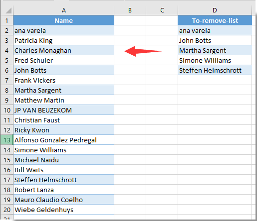
左側のスクリーンショットのように2 つのデータリストがあると仮定します。このとき、列 A 内の名前が列 D に存在する場合は、その名前を削除または除外したいもの。どのように実現すればよいでしょうか？また、2 つのリストが異なるワークシートにある場合はどうすればよいでしょうか？この記事では、そのための2 つの方法をご紹介します。

数式を使用してあるリストから別のリストの値を除外する

Kutools for Excel で素早くあるリストから別のリストの値を除外する

数式を使用してあるリストから別のリストの値を除外する

これを実現するには、以下の数式を適用してください。手順に従って進めてください。

1．削除したいリストの最初のセルの隣にある空白セルを選択し、数式バーに=COUNTIF($D$2:$D$6,A2)と入力して、Enterキーを押してください。スクリーンショットをご確認ください。

ヘルパー列を作成するために数式を入力する

注：この数式では、$D$2：$D$6 が値を削除する際の基準リストを示し、A2 は削除対象リストの先頭セルです。必要に応じて、これらの参照を適宜変更してください。

2．結果セルをそのまま選択した状態で、フィルハンドルをリストの末尾セルまでドラッグしてください。スクリーンショットをご参照ください。

数式を他のセルにドラッグしてコピーする

3．結果リストをそのまま選択した状態で、「データ>昇順」をクリックします。

[データ] > [昇順 (A から Z)] をクリックする

すると、以下のようなスクリーンショットのようにリストが並べ替えられます。

[並べ替え] ボタンをクリックする

4．次に、結果が1 である名前の行全体を選択し、右クリックして「削除」をクリックして削除してください。

結果が 1 である名前の行全体を選択し、削除する

これで、あるリストから別のリストに基づいて値を除外できました。

注：「削除対象リスト」が Sheet2 などの別のワークシートの A2:A6 範囲にある場合は、次の数式 =IF(ISERROR(VLOOKUP(A2,Sheet2!$A$2:$A$6,1,FALSE)),「Keep」,「Delete」)を適用して、すべての保持および削除結果を取得してください。その後、結果リストを A～Z の順に並べ替え、現在のワークシートで「削除」結果を含むすべての名前行を手動で削除してください。

Kutools for Excel で素早くあるリストから別のリストの値を除外する

このセクションでは、この問題を解決するために、同じ/異なるセルを選択機能（)Kutools for Excel）をおすすめします。以下の手順に従ってください。

Kutools for Excelは300 以上の高度な機能を提供し、複雑な作業を効率化して、創造性と生産性を高めます。AI 機能と統合されたKutools は、正確にタスクを自動化し、データ管理を簡単にします。Kutools for Excel の詳細情報。。。 無料トライアル。。。

1．「Kutools > 選択 > 同じ/異なるセルを選択」をクリックしてください。スクリーンショットをご覧ください。

Kutools の [同じセルと異なるセルを選択] 機能をクリックする

2．「同じ/異なるセルを選択」ダイアログボックスで、次の操作を行ってください。

2.1「次の値を検索する範囲」ボックスで、値を削除したいリストを選択します。
2.2「基準となるリスト」ボックスで、値を削除する際の基準とするリストを選択します。
2.3「単一セル」オプションを「基準」セクションで選択してください。
2.4「OK」ボタンをクリックしてください。スクリーンショットをご確認ください。

ダイアログボックスでオプションを設定する

3．その後、選択されたセルの数を示すダイアログボックスが表示されるので、「OK」ボタンをクリックしてください。

選択されたセルの数を知らせるダイアログボックスが表示される

4．これで、列 D に値が存在する場合、列 A の値が自動的に選択されます。手動で削除するには、Deleteキーを押してください。

Delete キーを押してそれらを削除する

このユーティリティの30 日間無料トライアルをご利用になりたい場合は、こちらをクリックしてダウンロードしてください。その後、上記の手順に従って操作を適用してください。

Kutools for Excel で素早くあるリストから別のリストの値を除外する

最高の Office 業務効率化ツール

🤖	KUTOOLS AI アシスタント：次に基づいてデータ分析を革新します：インテリジェント実行｜コード生成｜カスタム数式作成｜データ分析とチャート生成｜拡張機能呼び出し…
	人気の機能：検索・ハイライト、または重複をマーキング｜空白行を削除する｜データを失うことなく列の結合またはセルを｜数式を使用しない四捨五入...
	スーパー LOOKUP：複数条件 VLookup ｜複数値 VLookup ｜複数シート間 VLookup ｜ファジーマッチ....
	高度なドロップダウンリスト：ドロップダウンリストをすばやく作成｜連動型ドロップダウンリスト｜複数選択可能なドロップダウンリスト....
	列マネージャー：指定した数の列を追加｜列の移動｜非表示列の表示状態を切り替え｜範囲および列の比較...
	注目の機能：グリッドフォーカス｜デザインビュー｜強化された数式バー｜ワークブックとシートマネージャー｜リソースライブラリ（オートテキスト）｜日付ピッカー｜ワークシートの統合｜暗号化／セルの復号化｜リストからメール送信｜スーパーフィルター｜特殊フィルタ（太字のフォントを持つセルをフィルタリング／斜体／取り消し線。。。）。。。
	トップ15 ツールセット：12 テキストツール（テキストの追加、特定の文字を削除、...）｜ 50+チャートタイプ（ガントチャート、...）｜ 40+実用的関数（誕生日に基づいて年齢を計算します、...）｜ 19 挿入ツール（QR コードを挿入、パスから画像を挿入、...）｜ 12 変換ツール（単語に変換する、為替レートの変換、...）｜ 7 結合と分割ツール（高度な行のマージ、セルの分割、...）｜さらに多数

Kutools はお好みの言語でご利用いただけます。英語、スペイン語、ドイツ語、フランス語、中国語、および40+の他の言語をサポートしています！

Kutools for Excel でExcel スキルを強化し、これまでにない効率を体験しましょう。Kutools for Excel は、生産性を高め、時間を大幅に節約できる高度な機能を300 以上提供します。最も必要な機能を今すぐ入手するにはこちらをクリック。。。

Kutools for Excel の詳細はこちら。。。無料ダウンロード。。。

Office Tab は Office にタブインターフェースをもたらし、作業を大幅に簡単にします

Word、Excel、PowerPoint でタブを使った編集と閲覧を有効にします。Publisher、Access、Visio、Project でもご利用いただけます。
複数のドキュメントを、新しいウィンドウではなく、同じウィンドウ内の新しいタブで開いたり作成したりできます。
日々の生産性を50％も向上させ、毎日数百回ものマウスクリックを削減します！