Google Sheets で別のシートを基に条件付き書式を設定するにはどうすればよいですか?
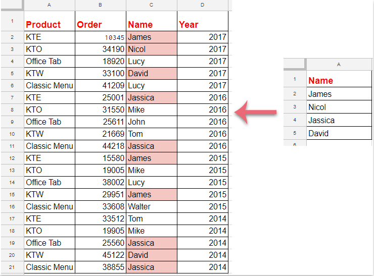
条件付き書式は Google Sheets の便利な機能で、特定の条件に基づいてセルを自動的にハイライトし、データの分析や可視化を簡単にします。同じシート内の値ではなく、別のシートに保存された参照リストや条件に基づいて書式ルールを設定したい場合もあるでしょう。たとえば、あるシートのセルが別のシートで管理されているリストに含まれているときにハイライトするといったケースです(下記のスクリーンショット参照)。このような操作は、現在の売上をマスタープロダクトリストと照合したり、別の範囲にある重複エントリをチェックしたりするなど、複数のシート間でデータを相互参照する際に頻繁に使われます。ただし、特にシートをまたいでデータを参照する条件付き書式の設定は、初めての方にとってはややこしく感じられるかもしれません。以下のガイドでは、この機能を実現するためのシンプルでわかりやすい手順をステップごとに説明します。
Google Sheets で別のシートのリストに基づいてセルをハイライトする方法
Google Sheets で別のシートのリストに基づいてセルをハイライトする方法
この方法では、別のシートにある指定リストに値が含まれている場合に、現在のワークシート内のセルをハイライトする条件付き書式ルールを設定できます。こうしたシート間の条件付き書式は、動的なデータ監視や関連データセット間の一貫性維持に特に役立ちます。
このプロセスを完了するには、以下の詳細な手順に従ってください。
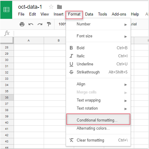
1。対象のワークシートを開き、画面上部の書式メニューをクリックして、条件付き書式を使用するを選択してください。すると、画面右側に条件付きフォーマットルールペインが表示されます。
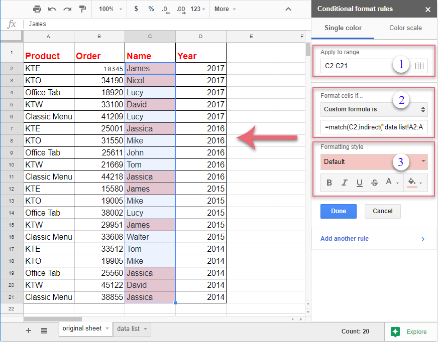
2。条件付きフォーマットルールパネルで、以下の操作を行ってください。
(1。)「範囲に適用」フィールド横の ボタンをクリックして、ハイライトしたいセル範囲を選択してください。たとえば、C 列の2 行目以降のすべての値に書式を適用する場合は、C2:Cを選択します。適切な範囲を指定すれば、意図したセルだけが書式評価の対象になります。
(2。)セルの書式設定の条件ドロップダウンメニューで、カスタム数式を使用を選択し、表示されたボックスに次の数式を入力します。=MATCH(C2,INDIRECT(「data list!A2:A」),0)。この数式は、「data list」シートの A2:A 範囲内に C 列の各セルの値が含まれているかどうかをチェックします。
(3。)書式スタイルで、セルの塗りつぶし色やフォントスタイルなど、好みの書式を自由に選べます。適用前に、シート上でスタイルを即座にプレビュー可能!
注:上記の数式において、C2は「範囲を選択してください」の最初のセルを指しています(データが別の行または列から始まる場合は、適宜調整してください)。また、data list!A2:Aは、リストが保存されているシート名(「data list」)とその対応する範囲(A2:A)を示しています。数式内のセル参照が、「範囲を選択してください」の左上セルと一致していることを必ずご確認ください。一致しない場合、書式が正しく適用されない可能性があります。データリストの範囲が異なる場合は、数式内を必ず更新してください(例:「data list!B2:B」)。
3。ルールを設定すると、選択した範囲内で他のシートのリストと一致するセルがすぐにハイライトされます。プレビューを確認したら、条件付きフォーマットルールペインの下部にある完了をクリックして、書式設定を適用・保存してください。
ヒントとトラブルシューティング:
- 数式内のタイポ(特にシート名や範囲の参照)を今一度ご確認ください。参照が誤っていると、ルールが適用されない原因となることがよくあります。
- データリストに空白セルが含まれている場合、
MATCH関数は一致しない値に対して#N/Aエラーを返します。これは想定された動作であり、一致する項目のハイライトには影響しません。 - 新しいシートに書式をコピーしたり範囲を調整したりした場合は、カスタム数式内のセル参照もそれに応じて更新してください。
- 後で参照リストに項目を追加または削除すると、書式設定が自動的に更新されます。
- 数式内で参照されているシートおよび範囲が実際に存在し、正しいスペルになっていること。
- 数式内の最初のセルが、「範囲を選択してください」で指定した最初のセルと一致していること。
- スプレッドシート内でのシート間アクセスに必要なすべての権限が利用可能であること。この方法は、単一の複数シートからなる Google Sheets ファイル内でのみ機能し、異なるファイル間では使用できません。
代替手段として、データ構造や要件がより複雑な場合(たとえば、複数列を比較したい、部分一致を許容したい、高度な検索を行いたいなど)には、COUNTIFまたはVLOOKUP 関数を使ったヘルパー列を作成するか、Google Apps Script(カスタム JavaScript コード)を活用することで、柔軟な条件付き書式設定を実現するソリューションも可能です。
まとめると、別のシートに基づいた条件付き書式を使用するの設定は、リスト照合、重複追跡、さまざまなシート間データ検証に非常に効果的です。これらはすべて Google Sheets 内で実現できます。常に数式の入力内容、参照範囲、書式ルールを確認し、スムーズかつ正確な結果を得るようにしてください。

KUTOOLS AI でExcel の魔法を解き放ちましょう
- スマート実行:セル操作、データ分析、チャート作成をすべてシンプルなコマンドで実現します。
- カスタム数式:ワークフローの効率化に役立つ、あなただけのカスタマイズ数式を生成します。
- VBA コーディング:VBA コードを簡単に記述・実装できます。
- 数式の解釈:複雑な数式が簡単に理解できます。
- テキスト翻訳:スプレッドシート内で言語の壁を乗り越えましょう!
最高の Office 業務効率化ツール
| 🤖 | KUTOOLS AI アシスタント:次に基づいてデータ分析を革新します:インテリジェント実行 | コード生成| カスタム数式作成 | データ分析とチャート生成| 拡張機能呼び出し… |
| 人気の機能:検索・ハイライト、または重複をマーキング | 空白行を削除する | データを失うことなく列の結合またはセルを | 数式を使用しない四捨五入... | |
| スーパー LOOKUP:複数条件 VLookup | 複数値 VLookup | 複数シート間 VLookup | ファジーマッチ.... | |
| 高度なドロップダウンリスト:ドロップダウンリストをすばやく作成 | 連動型ドロップダウンリスト | 複数選択可能なドロップダウンリスト.... | |
| 列マネージャー:指定した数の列を追加|列の移動|非表示列の表示状態を切り替え|範囲および列の比較... | |
| 注目の機能:グリッドフォーカス | デザインビュー |強化された数式バー | ワークブックとシートマネージャー | リソースライブラリ(オートテキスト)| 日付ピッカー | ワークシートの統合 | 暗号化/セルの復号化 | リストからメール送信 | スーパーフィルター | 特殊フィルタ(太字のフォントを持つセルをフィルタリング/斜体/取り消し線。。。) 。。。 | |
| トップ15 ツールセット:12 テキストツール(テキストの追加、特定の文字を削除、...)| 50+チャートタイプ(ガントチャート、...)| 40+実用的関数(誕生日に基づいて年齢を計算します、...)| 19 挿入ツール(QR コードを挿入、パスから画像を挿入、...)| 12 変換ツール(単語に変換する、為替レートの変換、...)| 7 結合と分割ツール(高度な行のマージ、セルの分割、...)|さらに多数 |
Kutools for Excel でExcel スキルを強化し、これまでにない効率を体験しましょう。Kutools for Excel は、生産性を高め、時間を大幅に節約できる高度な機能を300 以上提供します。最も必要な機能を今すぐ入手するにはこちらをクリック。。。
Office Tab は Office にタブインターフェースをもたらし、作業を大幅に簡単にします
- Word、Excel、PowerPoint でタブを使った編集と閲覧を有効にします。Publisher、Access、Visio、Project でもご利用いただけます。
- 複数のドキュメントを、新しいウィンドウではなく、同じウィンドウ内の新しいタブで開いたり作成したりできます。
- 日々の生産性を50%も向上させ、毎日数百回ものマウスクリックを削減します!
すべてのKutools アドインが、たった1 つのインストーラーで完結。
Kutools for Officeスイートには、Excel ・Word ・Outlook ・PowerPoint 用のアドインと Office Tab Pro が含まれており、複数の Office アプリを横断して作業するチームに最適です。
- オールインワンスイート— Excel、Word、Outlook、PowerPoint 用アドイン+Office Tab Pro
- インストーラー1 つ、ライセンス1 つ— 数分でセットアップ可能(MSI 対応)
- 連携してさらにパワーアップ— Office アプリ全体で生産性が向上
- 30 日間のフル機能トライアル— 登録不要、クレジットカード不要
- 最高のお得感— 個別アドイン購入よりお得