Excel のグラフ凡例で項目の順序を逆にするにはどうすればよいですか?
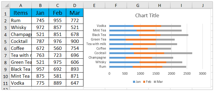
複雑なデータセットを扱う際、Excel でチャートを使って情報を可視化するのは一般的な手法であり、データの傾向を効果的に伝えるのに非常に役立ちます。たとえば、月次の売上データを含む売上表があり、下記のスクリーンショットのように積み上げ横棒グラフを作成してこの情報を表示しているとします。既定では、Excel はデータの最初のエントリ(例:1 月の売上)から凡例を表示し、その後に2 月、3 月と続き、多くの場合、データの時系列順と一致します。しかし、特定のレポート要件やより効果的な視覚的比較のために、この順序を逆にする必要が生じることがあります(例:チャートおよび凡例の両方で3 月を最初に、1 月を最後に表示するなど)。グラフ凡例内の項目の順序を逆にする方法を理解すれば、特定のニーズやプレゼンテーションの好みに合わせてレポートを柔軟に調整できます。本チュートリアルでは、Excel の積み上げ横棒グラフで凡例項目の順序を逆にするための詳細なステップ・バイ・ステップ手順をご紹介します。
Excel のグラフ凡例で項目の順序を逆にする
Excel 上で直接、積み上げ横棒グラフの凡例項目の表示順序を逆にしたい場合は、データ系列の配置を調整することで実現できます。凡例の順序を変更すれば、レポートの優先順位に沿った視覚化や、他のビジネス文書との整合性をよりスムーズに保つことが可能になります。以下では、凡例項目を上から下へと手動で並べ替える方法をご紹介します。
1。グラフ上の任意の場所を右クリックし、コンテキストメニューからSelect Dataを選択してください。すると、「データの選択」ダイアログボックスが開き、すべてのグラフ系列が一覧表示されます。![右クリックメニューの[データの選択]オプション](http://cdn.extendoffice.com/images/stories/doc-excel/chart-reverse-legend-order/doc-excel-chart-reverse-legend-order-2.png)
2。Legend Entries (Series)セクションに注目してください。最初の凡例項目(例:1 月)をクリックして選択し、Move Downボタンを使って![[データ ソースの選択]ダイアログ ボックス([下へ移動]ボタンが強調表示)](http://cdn.extendoffice.com/images/stories/doc-excel/chart-reverse-legend-order/doc-excel-chart-reverse-legend-order-3.png) 系列リストの一番下まで移動させます。
系列リストの一番下まで移動させます。
3。必要なだけこの操作を繰り返して、残りの各系列を下に移動させ、元々最後にあった系列がリストの先頭に来るようにしてください。系列の順序を変更すると、凡例の位置も即座に更新されます。完了したら、OKをクリックしてダイアログボックスを確定し、閉じます。![凡例が並べ替えられた[データ ソースの選択]ダイアログ ボックス](http://cdn.extendoffice.com/images/stories/doc-excel/chart-reverse-legend-order/doc-excel-chart-reverse-legend-order-5.png)
ワークシートに戻ると、グラフの凡例が逆順で表示されていることを確認できます。
ヒント:
- グラフに多くの系列が含まれている場合は、並べ替え中に混乱を避けるため、事前に系列ラベルをしっかり把握しておきましょう。変更を行う前に、初期の順序をメモしておくことをおすすめします。
- 手動で並べ替える際は、特に後で系列を追加または削除する場合に注意が必要です。変更後は凡例の順序を確認し、意図したとおりになっているかを必ずチェックしてください。
- グラフが動的範囲にリンクされている場合や定期的に更新される場合は、ソースデータを更新した後にこの手順を再度実行する必要がある場合があります。
トラブルシューティング:
- 「上へ移動」/「下へ移動」ボタンが使えない、またはグレーアウトしている場合は、リスト内のシリーズ名を直接クリックしてからボタンをお試しください。
- グラフに変更が反映されない場合は、ファイルを一度閉じて再度開くか、F9 キーを押して再計算(更新)してください。
関連記事:
最高の Office 業務効率化ツール
| 🤖 | KUTOOLS AI アシスタント:次に基づいてデータ分析を革新します:インテリジェント実行 | コード生成| カスタム数式作成 | データ分析とチャート生成| 拡張機能呼び出し… |
| 人気の機能:検索・ハイライト、または重複をマーキング | 空白行を削除する | データを失うことなく列の結合またはセルを | 数式を使用しない四捨五入... | |
| スーパー LOOKUP:複数条件 VLookup | 複数値 VLookup | 複数シート間 VLookup | ファジーマッチ.... | |
| 高度なドロップダウンリスト:ドロップダウンリストをすばやく作成 | 連動型ドロップダウンリスト | 複数選択可能なドロップダウンリスト.... | |
| 列マネージャー:指定した数の列を追加|列の移動|非表示列の表示状態を切り替え|範囲および列の比較... | |
| 注目の機能:グリッドフォーカス | デザインビュー |強化された数式バー | ワークブックとシートマネージャー | リソースライブラリ(オートテキスト)| 日付ピッカー | ワークシートの統合 | 暗号化/セルの復号化 | リストからメール送信 | スーパーフィルター | 特殊フィルタ(太字のフォントを持つセルをフィルタリング/斜体/取り消し線。。。) 。。。 | |
| トップ15 ツールセット:12 テキストツール(テキストの追加、特定の文字を削除、...)| 50+チャートタイプ(ガントチャート、...)| 40+実用的関数(誕生日に基づいて年齢を計算します、...)| 19 挿入ツール(QR コードを挿入、パスから画像を挿入、...)| 12 変換ツール(単語に変換する、為替レートの変換、...)| 7 結合と分割ツール(高度な行のマージ、セルの分割、...)|さらに多数 |
Kutools for Excel でExcel スキルを強化し、これまでにない効率を体験しましょう。Kutools for Excel は、生産性を高め、時間を大幅に節約できる高度な機能を300 以上提供します。最も必要な機能を今すぐ入手するにはこちらをクリック。。。
Office Tab は Office にタブインターフェースをもたらし、作業を大幅に簡単にします
- Word、Excel、PowerPoint でタブを使った編集と閲覧を有効にします。Publisher、Access、Visio、Project でもご利用いただけます。
- 複数のドキュメントを、新しいウィンドウではなく、同じウィンドウ内の新しいタブで開いたり作成したりできます。
- 日々の生産性を50%も向上させ、毎日数百回ものマウスクリックを削減します!
すべてのKutools アドインが、たった1 つのインストーラーで完結。
Kutools for Officeスイートには、Excel ・Word ・Outlook ・PowerPoint 用のアドインと Office Tab Pro が含まれており、複数の Office アプリを横断して作業するチームに最適です。
- オールインワンスイート— Excel、Word、Outlook、PowerPoint 用アドイン+Office Tab Pro
- インストーラー1 つ、ライセンス1 つ— 数分でセットアップ可能(MSI 対応)
- 連携してさらにパワーアップ— Office アプリ全体で生産性が向上
- 30 日間のフル機能トライアル— 登録不要、クレジットカード不要
- 最高のお得感— 個別アドイン購入よりお得