Excel でピボットテーブルのフィルターを特定のセルにリンクするにはどうすればよいですか？

著者Siluvia変更日2025-07-16

Excel では、特定のセルの値に基づいて PivotTable フィルターを自動更新するインタラクティブなレポートを作成したい場面がよくあります。これにより、ユーザーが1 か所でフィルター値を選択または入力するだけで、PivotTable がその入力に応じて動的に更新されます。この仕組みは、ダッシュボードやデータ探索用のフィルター設定インターフェースを構築する際に特に効果的です。

本記事では、VBA を活用したアプローチやExcel の標準機能を組み合わせた実用的な解決策をご紹介し、ピボットテーブルのフィルターをセルの値にリンクさせたり、同様の動的レポート効果を実現したりする方法をサポートします。

VBA コードを使用して PivotTable フィルターを特定のセルにリンクする
Excel 数式 – スライサーやレポートフィルターの参照と併用して数式（例：GETPIVOTDATA）を使用する
その他のExcel 標準機能 – インタラクティブなフィルタリングのために PivotTable スライサーとダッシュボードを接続する

VBA コードを使用して PivotTable フィルターを特定のセルにリンクする

セルの値を変更した際に自動的に PivotTable フィルターが更新されるよう、セルと PivotTable フィルターを最も直接的に連携させる必要がある場合は、VBA が実用的な手段を提供します。このアプローチは、ユーザーが1 つのセルからデータのスライスを素早く操作したいインタラクティブなダッシュボードやレポートに最適です。

このテクニックを正しく機能させるには、お使いのピボットテーブルにフィルターフィールドが含まれている必要があります。フィルターフィールドの名前は、VBA コードを適切に設定するうえで重要です。

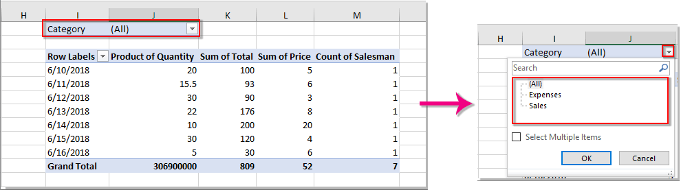
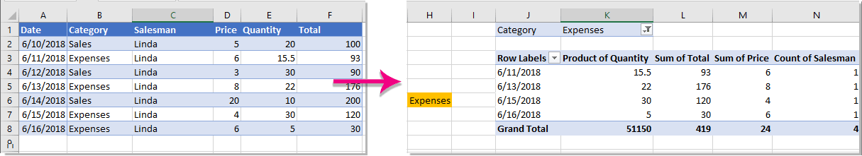
以下の例を考えてみましょう。Categoryという名前のフィルターフィールドを含む PivotTable があり、そのフィルター値には「Expenses」と「Sales」の2 つがあります。セルを PivotTable のフィルターにリンクすれば、そのセルに「Expenses」または「Sales」と入力するだけで、表示されるデータを自在にコントロールできます。

ピボットテーブルのフィルターを特定のセルにリンクする

これを実装する手順は次のとおりです。

フィルターのコントローラーとして使用するセル（例：セル H6）を選択し、事前にフィルター値のいずれかを入力してください。この値がピボットテーブルのフィルターフィールドで利用可能な値と完全に一致していることをご確認ください。
PivotTable を含むワークシートに移動し、シート見出しを右クリックしてメニューからコードの表示を選択してください。すると、Visual Basic for Applications ウィンドウが開きます。

シートタブを右クリックして［コードの表示］を選択

Microsoft Visual Basic for Applicationsウィンドウで、次の VBA コードをコードペインに貼り付けてください。

VBA コード：PivotTable フィルターを特定のセルにリンクする

Private Sub Worksheet_Change(ByVal Target As Range)
'Update by Extendoffice 20180702
    Dim xPTable As PivotTable
    Dim xPFile As PivotField
    Dim xStr As String
    On Error Resume Next
    If Intersect(Target, Range("H6")) Is Nothing Then Exit Sub
    Application.ScreenUpdating = False
    Set xPTable = Worksheets("Sheet1").PivotTables("PivotTable2")
    Set xPFile = xPTable.PivotFields("Category")
    xStr = Target.Text
    xPFile.ClearAllFilters
    xPFile.CurrentPage = xStr
    Application.ScreenUpdating = True
End Sub

注意点：

1)Sheet1はシート名です。必要に応じて変更してください。

2)PivotTable2は PivotTable の名前です。実際のテーブルに合わせて調整してください。

3) 「Category」はフィルター対象のフィールドです。テーブル内のフィールド名とスペルが一致していることを確認してください。

4)H6はフィルターにリンクされる参照セルです。必要に応じてセルアドレスを変更できます。ただし、そのセルには常にデータセット内に存在する有効なフィルター値が含まれているようにしてください。

コードを貼り付けたら、Alt + Qを押して VBA エディターウィンドウを閉じ、Excel に戻りましょう。

これで、ピボットテーブルのフィルター状態がセル H6 の内容によって制御されるようになります。セル H6 の値を「Sales」または「Expenses」に変更するだけで、ピボットテーブルの表示が即座に更新されます。問題が発生した場合は、参照セルの値がピボットテーブル内のフィルター項目と完全に一致していること、およびコード内で正しく名前が割り当てられていることを再度ご確認ください。

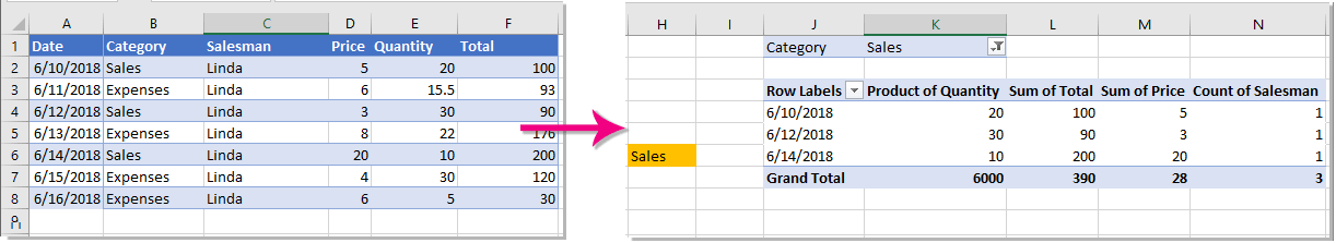
セルを更新すると、既存の値に基づいて対応するデータがフィルターで除外されます

セルの内容を変更するたびに、PivotTable はフィルターされたデータを自動的に更新します。

セルの値を変更すると、ピボットテーブル内のフィルターされたデータが自動的に変更されます。

ヒントとトラブルシューティング：セル内のフィルターフィールド値が利用可能な項目と（大文字・小文字やスペースを含めて）完全に一致しない場合、コードが期待通りにフィルターを適用できないことがあります。必ず、VBA コード内のフィールド名およびテーブル名のスペルが正確であることを確認してください。この設定を複数のピボットテーブルで使用する場合は、コードをさらに調整するか、ループ処理を追加して拡張できます。

KUTOOLS AI でExcel の魔法を解き放ちましょう

スマート実行：セル操作、データ分析、チャート作成をすべてシンプルなコマンドで実現します。
カスタム数式：ワークフローの効率化に役立つ、あなただけのカスタマイズ数式を生成します。
VBA コーディング：VBA コードを簡単に記述・実装できます。
数式の解釈：複雑な数式が簡単に理解できます。
テキスト翻訳：スプレッドシート内で言語の壁を乗り越えましょう！

AI 搭載のツールでExcel の機能をさらに強化しましょう。今すぐダウンロードして、これまでにない効率を体験してください！

Excel 数式 – スライサーやレポートフィルターの参照と併用して数式（例：GETPIVOTDATA）を使用する

Excel には、ピボットテーブルのフィルターをセルに直接バインドする純粋な数式ベースの標準機能はありませんが、GETPIVOTDATAなどの関数をスライサーやレポートフィルターと組み合わせることで、動的なレポートや関連する値の表示を実現できます。この手法は、フィルター選択や他のセルの入力に基づいて集計値が即座に更新されるダッシュボードを構築したいときに最適で、データ分析をよりインタラクティブにします。

適用可能なシナリオには、スライサーの選択に応じて表示内容が動的に変化するレポートパネル、ダッシュボード、比較サマリーなどが含まれます。この手法の最大のメリットは、最新のサマリーデータを表示するのに非常に適している点です。ただし、PivotTable の実際のフィルター状態をセルの数式のみでプログラム的に設定することはできません。

例：セルの値に基づく PivotTable サマリーの表示

たとえば、ピボットテーブルがCategory（例：「Sales」や「Expenses」）ごとの売上をサマリーしているとします。その場合、GETPIVOTDATAを使えば、セルで指定されたカテゴリに関連する値を簡単に抽出できます。

1。セル H6 に表示したいカテゴリ（例：「Sales」）が含まれていると仮定します。サマリーセル（例：I6）に次の数式を入力してください。

=GETPIVOTDATA("Sum of Amount",$B$4,"Category",H6)

2。I6 に数式を入力して Enter キーを押すと、H6 でカテゴリ（「Expenses」や「Sales」など）を変更するたびに、I6 が現在の PivotTable に基づいてそのカテゴリの合計を即座に表示するようになります。

注意点：

最初の引数「Sum of Amount」は、お使いのピボットテーブル内の値フィールドの実際の名前（例：「Total Sales」や、値に使用されているラベル）に置き換えてください。同様に、$B$4 はお使いのピボットテーブル内の特定のセルへの参照に置き換えてください。そうすることで、Excel が自動的にこの参照を認識し、GETPIVOTDATA 関数が正しいピボットテーブルと連携して正しく動作するようになります。
正確な GETPIVOTDATA 構文を取得するには、PivotTable 内のセルをクリックして値を参照してみてください。Excel が自動的に正しい構文を生成します。正確な結果を得るには、H6 の内容がテーブル内の利用可能なカテゴリのいずれかと一致していることをご確認ください。

ヒント：この方法では PivotTable 自体のフィルター状態は変更されませんが、セルがフィルターされたかのような効果で結果データを表示でき、ターゲットセルの入力に連動した動的な表示を実現します。チャート、サマリーテーブル、ダッシュボードの作成にも活用できます。

トラブルシューティング：#REF! エラーや#VALUE! エラーが表示された場合は、セル参照が正しいこと、入力したカテゴリがピボットテーブル内に存在すること、およびフィールド名／集計名が完全に一致していることをご確認ください。

その他のExcel 標準機能 – インタラクティブなフィルタリングのために PivotTable スライサーとダッシュボードを接続する

Excel のスライサーやレポートフィルターは、VBA コードを一切記述せずにインタラクティブなフィルタリングを実現できる、ユーザーフレンドリーな標準機能です。これらの機能を使えば、1 つまたは複数のスライサーを複数のピボットテーブルやビューに接続し、ダッシュボードのような効果を簡単に実現できます。

一般的なアプローチの1 つは、PivotTable フィールド（例：「Category」）にリンクしたスライサーを挿入することです。ユーザーがスライサー内の目的の項目をクリックするだけで、関連する PivotTable（複数可）が自動的に更新されます。同じソース範囲に基づく複数の PivotTable がある場合は、1 つのスライサーをすべてのテーブルに接続して同期フィルタリングを実現でき、レポートインターフェースがより直感的で一貫性のあるものになります。

スライサーを作成してリンクする手順は、次のとおりです。

お使いのピボットテーブル内をクリックし、ピボットテーブル分析（またはExcel のバージョンによっては)オプションタブ）を表示して、スライサーの挿入へ進みます。
目的のフィールド（例：Category）にチェックを入れて「OK」をクリックすると、スライサーがシート上に表示され、ユーザーが視覚的にフィルターをかけられるようになります。
1 つのスライサーを複数の PivotTable にリンクするには、スライサーを右クリックしてレポートの接続（または)ピボットテーブルの接続）を選択し、同期させたいすべての PivotTable にチェックを入れます。
ユーザーがフィルター操作を行うと、複数のビジュアライゼーションが即座に連動する——そんなダイナミックなダッシュボードを構築する際に特に効果的です。

メリット：ほとんどのインタラクティブなフィルタリング要件を、マクロやカスタムコードなしで非常に簡単に実現できます。シンプルさと信頼性が求められるダッシュボードや共有レポートに最適です。ただし、セルからフィルターへの完全な自動連携（セル値とフィルターの直接バインド）は標準機能ではサポートされておらず、セルの値を直接フィルターに割り当てるには VBA または外部ツールが必要です。

トラブルシューティング：スライサーが複数のピボットテーブルに接続されない場合は、すべてのテーブルが同じキャッシュ／ソース範囲に基づいて作成されていることを確認してください。レポートの接続オプションは、テーブル同士が互換性を持つ場合にのみ表示されます。

要約の提案：PivotTable フィルターをセル値にリンクする方法やインタラクティブなダッシュボードを構築する最適なアプローチを選ぶ際は、必要な自動化レベル、お使いのExcel のバージョンによる制限、およびご利用環境で VBA／マクロが許可されているかを慎重に検討してください。基本的な用途であれば、スライサーや GETPIVOTDATA 関数などの数式が、迅速かつ堅牢な結果をもたらします。一方、高度な自動化を求める場合は、VBA ソリューションがより高い制御性を実現します。正確な結果を得るには、常に条件名とフィルター項目が一貫して使用されていることを確認してください。エラーが発生した場合は、セルに入力された値を再確認し、コード・数式・データセット間で名称が完全に一致していることを保証してください。

最高の Office 業務効率化ツール

🤖	KUTOOLS AI アシスタント：次に基づいてデータ分析を革新します：インテリジェント実行｜コード生成｜カスタム数式作成｜データ分析とチャート生成｜拡張機能呼び出し…
	人気の機能：検索・ハイライト、または重複をマーキング｜空白行を削除する｜データを失うことなく列の結合またはセルを｜数式を使用しない四捨五入...
	スーパー LOOKUP：複数条件 VLookup ｜複数値 VLookup ｜複数シート間 VLookup ｜ファジーマッチ....
	高度なドロップダウンリスト：ドロップダウンリストをすばやく作成｜連動型ドロップダウンリスト｜複数選択可能なドロップダウンリスト....
	列マネージャー：指定した数の列を追加｜列の移動｜非表示列の表示状態を切り替え｜範囲および列の比較...
	注目の機能：グリッドフォーカス｜デザインビュー｜強化された数式バー｜ワークブックとシートマネージャー｜リソースライブラリ（オートテキスト）｜日付ピッカー｜ワークシートの統合｜暗号化／セルの復号化｜リストからメール送信｜スーパーフィルター｜特殊フィルタ（太字のフォントを持つセルをフィルタリング／斜体／取り消し線。。。）。。。
	トップ15 ツールセット：12 テキストツール（テキストの追加、特定の文字を削除、...）｜ 50+チャートタイプ（ガントチャート、...）｜ 40+実用的関数（誕生日に基づいて年齢を計算します、...）｜ 19 挿入ツール（QR コードを挿入、パスから画像を挿入、...）｜ 12 変換ツール（単語に変換する、為替レートの変換、...）｜ 7 結合と分割ツール（高度な行のマージ、セルの分割、...）｜さらに多数

Kutools はお好みの言語でご利用いただけます。英語、スペイン語、ドイツ語、フランス語、中国語、および40+の他の言語をサポートしています！

Kutools for Excel でExcel スキルを強化し、これまでにない効率を体験しましょう。Kutools for Excel は、生産性を高め、時間を大幅に節約できる高度な機能を300 以上提供します。最も必要な機能を今すぐ入手するにはこちらをクリック。。。

Kutools for Excel の詳細はこちら。。。無料ダウンロード。。。

Office Tab は Office にタブインターフェースをもたらし、作業を大幅に簡単にします

Word、Excel、PowerPoint でタブを使った編集と閲覧を有効にします。Publisher、Access、Visio、Project でもご利用いただけます。
複数のドキュメントを、新しいウィンドウではなく、同じウィンドウ内の新しいタブで開いたり作成したりできます。
日々の生産性を50％も向上させ、毎日数百回ものマウスクリックを削減します！