複数の条件に基づいてExcelで複数の一致する値を返す（完全ガイド）

Author Xiaoyang Last modified 2025-08-26

Excelユーザーは、複数の条件を同時に満たす複数の値を抽出し、すべての一致する結果を列、行、または単一のセルに統合して表示する必要があるシナリオによく遭遇します。このガイドでは、すべてのExcelバージョンでの方法と、Excel 365および2021で利用可能な新しいFILTER関数について説明します。

return multiple matching values based on criteria

単一のセル内で複数の条件に基づいて複数の一致する値を返す

Textjoin関数を使用（Excel365 / 2021, 2019）
Kutools for Excelを使用（すべてのバージョン対応）

列内で複数の条件に基づいて複数の一致する値を返す

配列数式を使用（すべてのバージョン対応）
Filter関数を使用（Excel365 / 2021）

行内で複数の条件に基づいて複数の一致する値を返す

配列数式を使用（すべてのバージョン対応）
Filter関数を使用（Excel365 / 2021）

単一のセル内で複数の条件に基づいて複数の一致する値を返す

Excelでは、単一のセル内で複数の条件に基づいて複数の一致する値を抽出することは一般的な課題です。ここでは、2つの効率的な方法を探ります。

方法1: Textjoin関数の使用（Excel365 / 2021,2019）

すべての一致する値を区切り文字付きで1つのセルに取得するには、TEXTJOIN関数が役立ちます。

次の数式を空白のセルにコピーまたは入力し、Enterキーを押します（Excel 2021およびExcel 365）。Excel 2019の場合はCtrl + Shift + Enterキーを押して結果を得ます：

=TEXTJOIN(", ", TRUE, IF(($A$2:$A$18=E2)*($B$2:$B$18=F2), $C$2:$C$18, ""))

Return multiple matching values based on multiple criteria in a single cell with textjoin function

この数式の説明：

($A$2:$A$21=E2)*($B$2:$B$21=F2) は、各行が「販売者がE2と等しい」および「月がF2と等しい」という両方の条件を満たしているかどうかを確認します。両方の条件が満たされた場合、結果は1、そうでない場合は0になります。アスタリスク * は、両方の条件が真であることを意味します。
IF(..., $C$2:$C$21, "") は、行が一致する場合、製品名を返します。それ以外の場合は空白を返します。
TEXTJOIN(", ", TRUE, ...) は、すべての非空白の製品名を", "で区切って1つのセルに結合します。

方法2: Kutools for Excelを使用

Kutools for Excelは、複雑な数式なしで複数の一致を素早く取得して1つのセルに結合できる強力かつシンプルなソリューションを提供します。

Kutools for Excelは、300以上の高度な機能を提供し、複雑なタスクを簡素化し、創造性と効率を向上させます。 AI機能と統合され、Kutoolsは正確にタスクを自動化し、データ管理を容易にします。Kutools for Excelの詳細情報...無料トライアル...

Kutools for Excelをインストール後、次の手順を行ってください：

基準に基づいてすべての対応する値を取得したいデータ範囲を選択します。
次に、Kutools > 結合 & 分割 > 高度な行のマージをクリックし、スクリーンショットをご覧ください：
高度な行のマージダイアログボックスで、以下のオプションを設定してください：
- 一致基準を含む列ヘッダー（例：販売者と月）を選択します。各選択した列に対して、Primary Keyをクリックして、これらを検索条件として定義します。
- 結合結果を取得したい列ヘッダー（例：製品）をクリックします。Combineセクションから、好みの区切り文字（例：カンマ、スペース、またはカスタム区切り文字）を選択します。
最後に、OKボタンをクリックします。

結果：Kutoolsは、一意の基準の組み合わせごとにすべての一致する値を即座に1つのセルにマージします。
Return multiple matching values based on multiple criteria in a single cell with kutools

列内で複数の条件に基づいて複数の一致する値を返す

いくつかの条件に基づいてデータセットから複数の一致するレコードを抽出して表示する必要があり、結果を縦方向の列形式で返す場合、Excelはいくつかの強力なソリューションを提供します。

方法1: 配列数式を使用（すべてのバージョン対応）

次の配列数式を使用して、結果を列に垂直に返すことができます：

1. 次の数式を空白のセルにコピーまたは入力します：

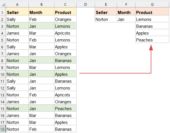
=IFERROR(INDEX($C$2:$C$18, SMALL(IF(($A$2:$A$18=$E$2)*($B$2:$B$18=$F$2), ROW($C$2:$C$18)-ROW($C$2)+1), ROW(1:1))), "")

2. 最初の一致する結果を得るためにCtrl + Shift + Enterキーを押し、最初の数式セルを選択し、空白のセルが表示されるまでフィルハンドルを下にドラッグします。これで、すべての一致する値が返されます（スクリーンショット参照）。

Return multiple matching values based on multiple criteria in a column with array formula

この数式の説明：

$A$2:$A$18=$E$2: 販売者がセルE2の値と一致するかチェックします。
$B$2:$B$18=$F$2: 月がセルF2の値と一致するかチェックします。
* は論理AND演算子（両方の条件が真である必要があります）。
ROW($C$2:$C$18)-ROW($C$2)+1: 各製品に対する相対行番号を生成します。
SMALL(..., ROW(1:1)): 数式を下にドラッグする際にn番目に小さい一致する行を取得します。
INDEX(...): 一致する行から製品を返します。
IFERROR(..., ""): 一致がなくなった場合、空白のセルを返します。

方法2: Filter関数を使用（Excel365 / 2021）

Excel 365またはExcel 2021を使用している場合、FILTER関数は、複雑な配列数式なしで結果を動的に展開できるため、複数の条件に基づいて複数の結果を返すのに最適な選択肢です。

次の数式を空白のセルにコピーまたは入力し、Enterキーを押すと、複数の基準に基づいてすべての一致するレコードが返されます。

=FILTER(C2:C18, (A2:A18=E2)*(B2:B18=F2), "No match")

Return multiple matching values based on multiple criteria in a column with filter function

この数式の説明：

FILTER(...) は、両方の条件が満たされている場合、C2:C18からすべての値を返します。
(A2:A18=E2)*(B2:B18=F2): 販売者と月が一致しているかチェックする論理配列。
"No match": 値が見つからない場合の任意のメッセージ。

行内で複数の条件に基づいて複数の一致する値を返す

Excelユーザーは、複数の条件を満たすデータセットから複数の値を抽出し、水平方向（行内）に表示する必要があります。これは、垂直方向のスペースが限られている動的レポート、ダッシュボード、または要約表を作成する際に役立ちます。このセクションでは、2つの強力な方法を探ります。

方法1: 配列数式を使用（すべてのバージョン対応）

従来の配列数式では、INDEX、SMALL、IF、COLUMN関数を使用して複数の一致する値を抽出できます。垂直方向の抽出（列ベース）とは異なり、数式を調整して結果を行に返します。

1. 次の数式を空白のセルにコピーまたは入力します：

=IFERROR(INDEX($C$2:$C$18, SMALL(IF(($A$2:$A$18=$E$2)*($B$2:$B$18=$F$2), ROW($C$2:$C$18)-ROW($C$2)+1), COLUMN(A1))), "")

2. 最初の一致する結果を得るためにCtrl + Shift + Enterキーを押し、最初の数式セルを選択し、数式を右にドラッグしてすべての結果を取得します。

Return multiple matching values based on multiple criteria in a row with array formula

この数式の説明：

$A$2:$A$18=$E$2: 販売者が一致するかチェックします。
$B$2:$B$18=$F$2: 月が一致するかチェックします。
*: 論理AND—両方の条件が真である必要があります。
ROW($C$2:$C$18)-ROW($C$2)+1: 相対行番号を作成します。
COLUMN(A1): 数式が右にドラッグされた距離に応じて、どの一致を返すか調整します。
IFERROR(...): 一致がなくなった際にエラーを防ぎます。

方法2: Filter関数を使用（Excel365 / 2021）

次の数式を空白のセルにコピーまたは入力し、Enterキーを押すと、すべての一致する値が抽出され、行に配置されます。スクリーンショットをご覧ください：

=TRANSPOSE(FILTER(C2:C18, (A2:A18=E2)*(B2:B18=F2), "No match"))

Return multiple matching values based on multiple criteria in a row with filter function

この数式の説明：

FILTER(...): 2つの条件に基づいて列Cから一致する値を取得します。
(A2:A18=E2)*(B2:B18=F2): 両方の条件が真である必要があります。
TRANSPOSE(...): FILTERによって返される垂直配列を水平配列に変換します。

conclusion

Excelで複数の条件に基づいて複数の一致する値を取得することは、結果を列、行、または単一のセルに表示するかによって、いくつかの方法で達成できます。

Excel 365またはExcel 2021を使用しているユーザーの場合、FILTER関数は現代的で動的かつ洗練されたソリューションを提供し、複雑さを最小限に抑えます。
古いバージョンを使用している場合、配列数式は依然として強力なツールですが、少し多くの設定と注意が必要です。
さらに、結果を1つのセルに統合したい場合やノーコードのソリューションを好む場合、TEXTJOIN関数やKutools for Excelのようなサードパーティツールがプロセスを大幅に簡素化します。

お使いのExcelのバージョンと希望するレイアウトに最も適した方法を選択すれば、複数条件の検索を効率的かつ正確に処理することができます。さらに多くのExcelのヒントやテクニックに関心がある場合は、当社のウェブサイトにはExcelをマスターするための数千のチュートリアルがあります。

Return Multiple Lookup Values In One Comma Separated Cell
Excelでは、VLOOKUP関数を使用してテーブルセルから最初に一致する値を返すことができますが、時にはすべての一致する値を抽出し、特定の区切り文字（カンマ、ダッシュなど）で区切って1つのセルにまとめる必要があります。Excelで複数の検索値を1つのカンマ区切りのセルに取得して返すにはどうすればよいですか？

Vlookup And Return Multiple Matching Values At Once In Google Sheet
Googleスプレッドシートでは、通常のVlookup関数を使用して指定されたデータに基づいて最初に一致する値を見つけて返すことができます。ただし、時々、すべての一致する値を返す必要がある場合があります。このタスクをGoogleスプレッドシートで解決する良い簡単な方法はありますか？

Vlookup And Return Multiple Values From Drop Down List
Excelでは、ドロップダウンリストから複数の対応する値をvlookupして返す方法は？つまり、ドロップダウンリストから項目を選択すると、そのすべての関連値が一度に表示されます（スクリーンショット参照）。この記事では、ステップバイステップで解決策を紹介します。

Vlookup And Return Multiple Values Vertically In Excel
通常、最初に対応する値を取得するためにVlookup関数を使用できますが、時には特定の基準に基づいてすべての一致するレコードを返したい場合があります。この記事では、すべての一致する値を垂直、水平、または1つのセルに返す方法について説明します。

Vlookup And Return Matching Data Between Two Values In Excel
Excelでは、与えられたデータに基づいて対応する値を取得するために通常のVlookup関数を使用できます。しかし、時々、2つの値の間で一致する値をvlookupして返したい場合があります（スクリーンショット参照）。このタスクをExcelでどのように処理できますか？

最高のオフィス業務効率化ツール

🤖	Kutools AI Aide：データ分析を革新します。主な機能：Intelligent Execution｜コード生成｜カスタム数式の作成｜データの分析とグラフの生成｜Kutools Functionsの呼び出し……
	人気の機能：重複の検索・ハイライト・重複をマーキング｜空白行を削除｜データを失わずに列またはセルを統合｜丸める……
	スーパーLOOKUP：複数条件でのVLookup｜複数値でのVLookup｜複数シートの検索｜ファジーマッチ……
	高度なドロップダウンリスト：ドロップダウンリストを素早く作成｜連動ドロップダウンリスト｜複数選択ドロップダウンリスト……
	列マネージャー：指定した数の列を追加｜列の移動｜非表示列の表示/非表示の切替｜範囲＆列の比較……
	注目の機能：グリッドフォーカス｜デザインビュー｜強化された数式バー｜ワークブック＆ワークシートの管理｜オートテキストライブラリ｜日付ピッカー｜データの統合｜セルの暗号化/復号化｜リストで電子メールを送信｜スーパーフィルター｜特殊フィルタ（太字/斜体/取り消し線などをフィルター）……
	トップ15ツールセット：12 種類のテキストツール（テキストの追加、特定の文字を削除など）｜50種類以上のグラフ（ガントチャートなど）｜40種類以上の便利な数式（誕生日に基づいて年齢を計算するなど）｜19 種類の挿入ツール（QRコードの挿入、パスから画像の挿入など）｜12 種類の変換ツール（単語に変換する、通貨変換など）｜7種の統合＆分割ツール（高度な行のマージ、セルの分割など）｜… その他多数