Excel でセルの値に基づいて背景色やフォント色を変更するにはどうすればよいですか?
Excel で大量のデータを扱う際、特定の値を抽出して背景色やフォント色で目立たせたいことがあります。本記事では、セルの値に基づいて背景色やフォント色を素早く変更する方法をご紹介します。
方法1:条件付き書式を使用するを使ってセルの値に基づき動的に背景色またはフォント色を変更する
条件付き書式を使用する機能を使えば、x より大きい値や y より小さい値、さらには x と y の間の値を簡単にハイライト表示できます。
大量のデータの中から80~100 の値に色付けしたい場合は、次の手順で操作してください。
1.ハイライトしたいセル範囲を選択し、次にホーム>条件付き書式を使用する>新しいルールをクリックします(下記スクリーンショット参照)。
![[ホーム]>[条件付き書式]>[新しいルール]をクリック](http://cdn.extendoffice.com/images/stories/doc-excel/change-fill-color/doc-highlight-by-value-1.png)
2.新しい書式設定のルールダイアログボックスで、ルールの種類の選択ボックスから指定した値を含むセルのみを書式設定するを選択し、次のセルのみを書式設定するセクションで必要な条件を設定してください。
- 最初のドロップダウンボックスでセルの値を選択してください。
- 2 番目のドロップダウンボックスで、次の範囲内という条件を選択します。
- 3 番目と4 番目のボックスにフィルター条件(例:80、100)を入力してください。

3.次に、書式設定ボタンをクリックして、セルの書式設定ダイアログボックスで背景色またはフォント色を次のように設定します。
| セルの値に基づいて背景色を変更します: | セルの値に基づいてフォント色を変更します |
| クリックして塗りつぶしタブを開き、お好みの背景色を選択してください | クリックしてフォントタブを開いて、必要なフォント色を選んでください。 |
![[塗りつぶし]タブで背景色を変更](http://cdn.extendoffice.com/images/stories/doc-excel/change-fill-color/doc-highlight-by-value-3.png) | ![[フォント]タブでフォントの色を変更](http://cdn.extendoffice.com/images/stories/doc-excel/change-fill-color/doc-highlight-by-value-4.png) |
4。 背景色またはフォント色を選択した後、OK>OKをクリックしてダイアログを閉じます。すると、選択範囲内で値が80 から100 の間にあるセルが、指定した背景色またはフォント色に自動的に変更されます(下記スクリーンショット参照)。
| 背景色で特定のセルをハイライト表示します: | フォント色で特定のセルをハイライト表示します: |
 |  |
注:条件付き書式を使用するは動的機能で、データが変更されるとセルの色が自動的に更新されます。
方法2:「検索」機能を使ってセルの値に基づき静的に背景色またはフォント色を変更する
セルの値に基づいて特定の塗りつぶし色やフォント色を固定したい場合があります。たとえば、セルの値が変更されてもその色が変わらないように設定したいときなどです。そんなときは、検索機能を使って該当するセルをすべて探し出し、その後、背景色やフォント色を目的の色に一括で変更しましょう。
たとえば、セルの値に「Excel」というテキストが含まれている場合に、背景色やフォント色を変更したいときは、次のように操作してください。
1.使用したいデータ範囲を選択し、次にホーム>検索と選択>検索をクリックします(下記スクリーンショット参照)。
![[ホーム]>[検索と選択]>[検索]をクリック](http://cdn.extendoffice.com/images/stories/doc-excel/change-fill-color/doc-highlight-by-value-7.png)
2.検索と置換ダイアログボックスで、検索タブの検索する文字列テキストボックスに、検索したい値を入力してください(下記スクリーンショット参照)。
![[検索する文字列]テキスト ボックスに検索する値を入力](http://cdn.extendoffice.com/images/stories/doc-excel/change-fill-color/doc-highlight-by-value-8.png)
3.次に、すべて検索ボタンをクリックし、検索結果ボックス内の任意の項目をクリックした後、Ctrl + Aキーを押してすべての検索結果を選択します(下記スクリーンショット参照)。

4.最後に、閉じるボタンをクリックしてこのダイアログを閉じると、選択されたセルに背景色またはフォント色が適用されます(下記スクリーンショット参照)。
| 選択したセルに背景色を適用します: | 選択したセルにフォント色を適用します: |
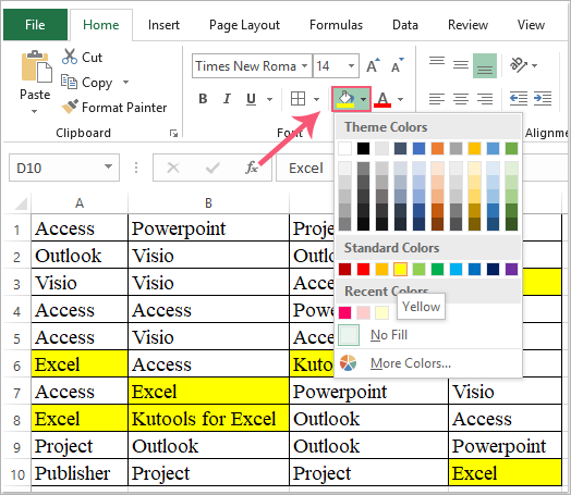 |  |
方法3:Kutools for Excel を使ってセルの値に基づき静的に背景色またはフォント色を変更する
Kutools for Excelのスーパー検索機能は、値、テキスト文字列、日付、数式、書式設定されたセルなど、さまざまな条件での検索をサポートしています。一致するセルを検索・選択した後は、背景色やフォント色を好みの色に簡単に変更できます。
1.検索したいデータ範囲を選択し、次にKutools>スーパー検索をクリックしてください(下記スクリーンショット参照)。

2.スーパー検索ペインで、次の操作を行ってください。
- (1)まず、値オプションのアイコンをクリックします。
- (2)対象範囲ドロップダウンから検索範囲を選択します。ここでは選択範囲を選びましょう。
- (3)種類ドロップダウンリストから、使用したい条件を選択します。
- (4)次に、検索ボタンをクリックすると、該当するすべての結果がリストボックスに表示されます。
- (5)最後に、選択ボタンをクリックしてセルを選択してください。

3.これで、条件に一致するすべてのセルが一括で選択されました(下記スクリーンショット参照)。

4.これで、選択したセルの背景色やフォント色を必要に応じて自由に変更できます。
最高の Office 業務効率化ツール
| 🤖 | KUTOOLS AI アシスタント:次に基づいてデータ分析を革新します:インテリジェント実行 | コード生成| カスタム数式作成 | データ分析とチャート生成| 拡張機能呼び出し… |
| 人気の機能:検索・ハイライト、または重複をマーキング | 空白行を削除する | データを失うことなく列の結合またはセルを | 数式を使用しない四捨五入... | |
| スーパー LOOKUP:複数条件 VLookup | 複数値 VLookup | 複数シート間 VLookup | ファジーマッチ.... | |
| 高度なドロップダウンリスト:ドロップダウンリストをすばやく作成 | 連動型ドロップダウンリスト | 複数選択可能なドロップダウンリスト.... | |
| 列マネージャー:指定した数の列を追加|列の移動|非表示列の表示状態を切り替え|範囲および列の比較... | |
| 注目の機能:グリッドフォーカス | デザインビュー |強化された数式バー | ワークブックとシートマネージャー | リソースライブラリ(オートテキスト)| 日付ピッカー | ワークシートの統合 | 暗号化/セルの復号化 | リストからメール送信 | スーパーフィルター | 特殊フィルタ(太字のフォントを持つセルをフィルタリング/斜体/取り消し線。。。) 。。。 | |
| トップ15 ツールセット:12 テキストツール(テキストの追加、特定の文字を削除、...)| 50+チャートタイプ(ガントチャート、...)| 40+実用的関数(誕生日に基づいて年齢を計算します、...)| 19 挿入ツール(QR コードを挿入、パスから画像を挿入、...)| 12 変換ツール(単語に変換する、為替レートの変換、...)| 7 結合と分割ツール(高度な行のマージ、セルの分割、...)|さらに多数 |
Kutools for Excel でExcel スキルを強化し、これまでにない効率を体験しましょう。Kutools for Excel は、生産性を高め、時間を大幅に節約できる高度な機能を300 以上提供します。最も必要な機能を今すぐ入手するにはこちらをクリック。。。
Office Tab は Office にタブインターフェースをもたらし、作業を大幅に簡単にします
- Word、Excel、PowerPoint でタブを使った編集と閲覧を有効にします。Publisher、Access、Visio、Project でもご利用いただけます。
- 複数のドキュメントを、新しいウィンドウではなく、同じウィンドウ内の新しいタブで開いたり作成したりできます。
- 日々の生産性を50%も向上させ、毎日数百回ものマウスクリックを削減します!
すべてのKutools アドインが、たった1 つのインストーラーで完結。
Kutools for Officeスイートには、Excel ・Word ・Outlook ・PowerPoint 用のアドインと Office Tab Pro が含まれており、複数の Office アプリを横断して作業するチームに最適です。
- オールインワンスイート— Excel、Word、Outlook、PowerPoint 用アドイン+Office Tab Pro
- インストーラー1 つ、ライセンス1 つ— 数分でセットアップ可能(MSI 対応)
- 連携してさらにパワーアップ— Office アプリ全体で生産性が向上
- 30 日間のフル機能トライアル— 登録不要、クレジットカード不要
- 最高のお得感— 個別アドイン購入よりお得