Microsoft Excel で動的データを並べ替えるには、どうすればよいですか？

文房具店の在庫記録など、常に変化するデータセットを管理する際には、正確なレポート作成や迅速な分析のために情報を効率的に並べ替えることが不可欠です。しかし、更新のたびに手動でデータを再並べ替えするのは、時間と手間がかかり、ミスも起こりやすくなります。そこで課題が生じます。基になるデータ（数量の調整や新規エントリーなど）が変更された際に、手動操作なしで最新の情報が常に反映されるよう、Excel のリストを自動的に並べ替えるにはどうすればよいでしょうか？

本記事では、Excel で動的データを自動的に並べ替えるための実践的な方法を詳しく解説します。数式を活用したアプローチ、VBA による自動化、そしてデータの変化に即応してテーブルを自動並べ替えできる最新のExcel 内蔵ツールをご紹介。これらの手法は、在庫管理、売上追跡、成績評価など、常に最新の順序でデータを把握したいあらゆる業務に最適です。

数式を使ってExcel で動的データを並べ替える

この方法は、すべての最新版Excel で動作し、元のテーブルの横に自動更新される並べ替え済みのコピーを常に維持したい場合に最適です。このアプローチでは順位を割り当て、その順位に基づいて値を検索するため、入力データが変更されても並べ替え済みテーブルは常に最新の状態を保ちます。

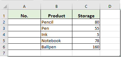
たとえば、複数の文房具アイテムの在庫数量を管理しているとします。数量を変更した際に即座に反映され、かつ在庫数量の降順で製品が表示されるようにするには、次の手順に従ってください。

1。 元のデータセットの先頭に新しい列を挿入します。サンプルドキュメントとシナリオでは、「No.」というタイトルの列を元データの前に挿入してください（下図参照）。

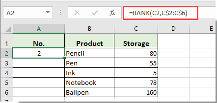
2。セル A2（「No.」の直下のセル。元データが A2:C6 であると仮定）に、保管数量に基づいて各製品の順位を計算する次の数式を入力してください。これにより、Excel は保管数量フィールドを使って各アイテムに一意の順位を割り当てます。

=RANK(C2, C$2:C$6)

数式を入力したら、Enterキーを押してください。RANK 関数は C2 の保管数量を C2:C6 の全範囲と比較し、順位を割り当てます（)1が最も保管数量が多い順位です）。アイテムが5 個を超える場合は、C6を必要な範囲に合わせて調整してください。

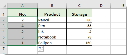
3。セル A2 を選択したまま、フィルハンドルをセル A6（またはデータの最終行）までドラッグして、リスト内のすべてのアイテムに順位付けの数式を適用します。

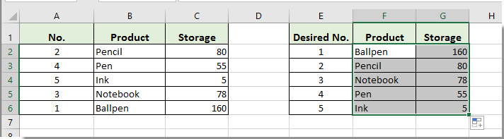
4。 動的に並べ替えられたテーブルを作成するには、まず元データのヘッダー行をコピーし、新しい場所（例：E1:G1）に貼り付けます。次に、新しい「希望順位」列（この例では E2:E6）に、順位に対応する連続した数値（1、2、3、…）を入力してください。この数列が取得順序を決定します。

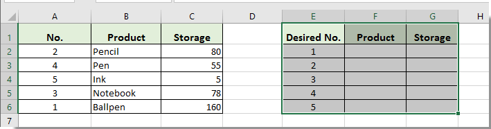
5。 新しいテーブルの「製品」列のセル F2 に、次の VLOOKUP 数式を入力して各順位番号に対応する製品名を取得し、Enterキーを押してください。

=VLOOKUP(E2, A$2:C$6, 2, FALSE)

この数式は、列 A で指定された順位を検索し、対応する製品名を第2 列から返します。

6。F2 から F6 までフィルハンドルをドラッグして、すべての製品名を入力します。並べ替え済みの保管数量を入力するには、F2:F6 を選択し、フィルハンドルを右に G2:G6 までドラッグします。

新しいテーブルでは、製品が保管数量の降順で表示され、常に元のテーブルの変更内容をリアルタイムに反映します。

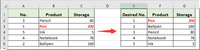
たとえば、文房具店で商品が入荷し、「ペン」の在庫数量を元のリストで55から200に更新すると、並べ替え済みの表では「ペン」のエントリが即座に新しい順位と数量を反映した位置に自動的に移動します。手動での並べ替えは一切不要！この仕組みにより、リストのメンテナンスが自動化され、手作業によるミスを削減しながら、重要なレポートの正確性をしっかり維持できます。

ヒントとトラブルシューティング：元のリストのサイズを変更した後は、新しく追加または削除されたアイテムがすべて数式の参照範囲に正しく含まれているか、再度確認してください。リストを拡張する際には、参照範囲を調整する必要がある場合があります（例：C$2:C$10ではなくC$2:C$6）。リストのサイズが頻繁に変わる場合は、データをExcel テーブルに変換し、セル範囲ではなくテーブルの列名で参照することをおすすめします。

ワークシート変更イベント（VBA）を使用してデータを自動的に並べ替える

この方法は、元の表を常に並べ替えられた状態に保ちたい場合に最適です。ユーザーがデータを編集したり新しいエントリを追加したりすると、その行は即座に再並べ替えられます。手動での並べ替え作業を減らし、共有リストや在庫ログなど頻繁に更新される記録にぴったりです。

メリット：ソースデータを常に並べ替えた状態に保つことができます。追加の表やコピーは不要で、列数を問わず対応可能です。

デメリット：マクロが必要です。このファイルを編集するすべてのユーザーが、マクロを有効にしたExcel を使用している必要があります。

使用例：ある文房具店が在庫を表で管理しています。在庫数量が変更されると、対応する行が自動的に正しい順位に並び替えられます。

ご注意ください：この方法はデータのレイアウトに直接影響を与えるため、必要に応じてバックアップやバージョン管理を事前に行ってください。

実装手順：

1。 自動並べ替えを適用したいシートタブを右クリックし、コードの表示を選択してください。

2。ワークシートのコードウィンドウ（標準モジュールではなく）に、次のコードを貼り付けてください。

Private Sub Worksheet_Change(ByVal Target As Range)
    On Error Resume Next
    Dim SortRange As Range
    ' Adjust your range as appropriate (example: A1:C6 includes headers)
    Set SortRange = Range("A1:C6")
    ' Sort by Storage in descending order (assuming Storage is in column C)
    SortRange.Sort Key1:=SortRange.Columns(3), Order1:=xlDescending, Header:=xlYes
End Sub

3。VBA エディターを閉じると、A1:C6の範囲内でデータが変更されるたびに、Excel が「在庫」列（列 C）を基準に降順で自動的に並べ替えを行います。

パラメーターの説明とトラブルシューティング：このマクロは、ヘッダー行が存在することを前提に、指定された固定範囲内で選択した列を並べ替えます。並べ替えが実行されない場合は、マクロが有効になっており、コードが正しいシートモジュールに配置されているかをご確認ください。また、ユーザーが制限された範囲外を編集した場合には並べ替えはトリガーされませんので、編集可能なすべての行をカバーするよう範囲を調整してください。

Excel テーブル（「テーブルとして書式設定」）を使用して簡単に並べ替える

データ範囲をテーブルとして書式設定機能で正式なExcel テーブルに変換すれば、リストの管理や並べ替えがぐっと快適になります！

典型的な使用例：共同作業用のワークブックや大規模なデータセットで、視覚的な整理と素早い行挿入が必要な場合、Excel テーブルを使えば日常的な並べ替えが簡単になり、ミスも減らせます。

使用方法：

1. データ範囲を選択し、Ctrl + Tを押してExcel テーブルに変換してください。このとき、「テーブルにヘッダーがあります」にチェックが入っていることを必ず確認しましょう。
2. 並べ替えたい列のヘッダーにあるドロップダウン矢印をクリックし（例：保管数量）、最大から最小へ順に並べ替えまたは最小から最大へ順に並べ替えを選択してください。

テーブルを編集するたびに自動的に並べ替えを実行したい場合は、前述の方法で VBA マクロをテーブルを含むシートにアタッチしてください。これにより、Excel テーブルの使いやすさと VBA による自動化を効果的に組み合わせることができます。

SORT 関数または SORTBY 関数（ダイナミック配列関数）を使用して並べ替える（Excel 365/2019+）

最新版のExcel（Excel 365、Excel 2019 以降）にはダイナミック配列関数が搭載されており、ヘルパー列や VBA を一切使わずに、リアルタイムで並べ替え済みのデータを自動生成できます。

使用例：ダッシュボード表示やレポート作成の際に、入力順序を編集やデータ入力用に保持しながら、常に最新の並べ替え済み在庫リストをライブで表示したい場合です。

使用方法：

元のデータテーブルが範囲 A2:C6にあり、ヘッダーがA1:C1にあると仮定します。「在庫」列（)Storage）を基準に降順で動的に並べ替えたテーブルを生成するには、たとえば空のセルE2に次の数式を入力してください。

=SORT(A2:C6, 3, -1)

これにより、元のテーブルの新しい並べ替え済みバージョンが生成され、3 列目（)Storage）を基準に降順で並べ替えられます。降順には-1、昇順には1を使用します。

より細かい並べ替え条件（複数キーでの並べ替えやカスタム条件など）を設定するには、SORTBYをご利用ください。

=SORTBY(A2:C6, C2:C6, -1, B2:B6, 1)

この数式では、まずStorageを降順で並べ替え、次にProductを昇順で並べ替えます。

数式を入力したら、Enterキーを押してください。Excel は並べ替えられたデータを隣接する行と列に「スピル」表示し、ソースデータが変更されると自動的にサイズを調整します。

これらのダイナミック配列関数を使えば、レポートやダッシュボード向けの大規模リストの並べ替えと更新が簡単に。出力は常に最新の状態を保ち、追加の手順は一切不要です。

KUTOOLS AI でExcel の魔法を解き放ちましょう

• スマート実行：セル操作、データ分析、チャート作成をすべてシンプルなコマンドで実現します。
• カスタム数式：ワークフローの効率化に役立つ、あなただけのカスタマイズ数式を生成します。
• VBA コーディング：VBA コードを簡単に記述・実装できます。
• 数式の解釈：複雑な数式が簡単に理解できます。
• テキスト翻訳：スプレッドシート内で言語の壁を乗り越えましょう！

AI 搭載のツールでExcel の機能をさらに強化しましょう。今すぐダウンロードして、これまでにない効率を体験してください！

最高の Office 業務効率化ツール

🤖	KUTOOLS AI アシスタント：次に基づいてデータ分析を革新します：インテリジェント実行   ｜  コード生成｜  カスタム数式作成  ｜  データ分析とチャート生成｜  拡張機能呼び出し…
	人気の機能：検索・ハイライト、または重複をマーキング   ｜  空白行を削除する   ｜  データを失うことなく列の結合またはセルを   ｜  数式を使用しない四捨五入...
	スーパー LOOKUP：複数条件 VLookup  ｜  複数値 VLookup  ｜   複数シート間 VLookup   ｜   ファジーマッチ....
	高度なドロップダウンリスト：ドロップダウンリストをすばやく作成   ｜  連動型ドロップダウンリスト   ｜  複数選択可能なドロップダウンリスト....
	列マネージャー：指定した数の列を追加｜列の移動｜非表示列の表示状態を切り替え｜範囲および列の比較...
	注目の機能：グリッドフォーカス   ｜  デザインビュー   ｜強化された数式バー   ｜ ワークブックとシートマネージャー   ｜  リソースライブラリ（オートテキスト）｜  日付ピッカー   ｜  ワークシートの統合  ｜  暗号化／セルの復号化   ｜ リストからメール送信   ｜  スーパーフィルター   ｜   特殊フィルタ（太字のフォントを持つセルをフィルタリング／斜体／取り消し線。。。） 。。。
	トップ15 ツールセット：12 テキストツール（テキストの追加、特定の文字を削除、...）｜   50+チャートタイプ（ガントチャート、...）｜   40+実用的関数（誕生日に基づいて年齢を計算します、...）｜   19 挿入ツール（QR コードを挿入、パスから画像を挿入、...）｜   12 変換ツール（単語に変換する、為替レートの変換、...）｜   7 結合と分割ツール（高度な行のマージ、セルの分割、...）｜さらに多数

Kutools はお好みの言語でご利用いただけます。英語、スペイン語、ドイツ語、フランス語、中国語、および40+の他の言語をサポートしています！

Kutools for Excel でExcel スキルを強化し、これまでにない効率を体験しましょう。Kutools for Excel は、生産性を高め、時間を大幅に節約できる高度な機能を300 以上提供します。最も必要な機能を今すぐ入手するにはこちらをクリック。。。

Kutools for Excel の詳細はこちら。。。無料ダウンロード。。。

---

Office Tab は Office にタブインターフェースをもたらし、作業を大幅に簡単にします

• Word、Excel、PowerPoint でタブを使った編集と閲覧を有効にします。Publisher、Access、Visio、Project でもご利用いただけます。
• 複数のドキュメントを、新しいウィンドウではなく、同じウィンドウ内の新しいタブで開いたり作成したりできます。
• 日々の生産性を50％も向上させ、毎日数百回ものマウスクリックを削減します！

Office Tab の詳細はこちら。。。無料ダウンロード。。。

---

すべてのKutools アドインが、たった1 つのインストーラーで完結。

Kutools for Officeスイートには、Excel ・Word ・Outlook ・PowerPoint 用のアドインと Office Tab Pro が含まれており、複数の Office アプリを横断して作業するチームに最適です。

• オールインワンスイート— Excel、Word、Outlook、PowerPoint 用アドイン＋Office Tab Pro
• インストーラー1 つ、ライセンス1 つ— 数分でセットアップ可能（MSI 対応）
• 連携してさらにパワーアップ— Office アプリ全体で生産性が向上
• 30 日間のフル機能トライアル— 登録不要、クレジットカード不要
• 最高のお得感— 個別アドイン購入よりお得

Kutools for Office の詳細はこちら。。。無料ダウンロード。。。