メインコンテンツへスキップ

Excelの列と行の基準に基づいて合計する方法は? 

著者:シャオヤン 最終更新日:2020年11月18日

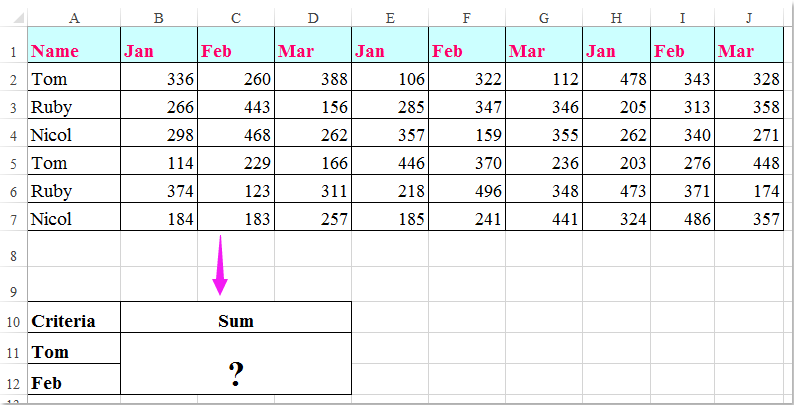
行ヘッダーと列ヘッダーを含むデータの範囲があります。次に、列ヘッダーと行ヘッダーの両方の条件を満たすセルの合計を取得します。 たとえば、次のスクリーンショットに示すように、列の基準がTomで、行の基準がFebであるセルを合計します。 この記事では、それを解決するためのいくつかの便利な式について説明します。

ドキュメントの合計列の行の基準1

数式を使用して列と行の基準に基づいてセルを合計する


矢印青い右バブル 数式を使用して列と行の基準に基づいてセルを合計する

ここでは、次の数式を適用して、列と行の両方の基準に基づいてセルを合計できます。次のようにしてください。

結果を出力する空白のセルに、次の数式のいずれかを入力します。

=SUMPRODUCT((A2:A7="Tom")*(B1:J1="Feb")*(B2:J7))

=SUM(IF(B1:J1="Feb",IF(A2:A7="Tom",B2:J7)))

そして、 Shift + Ctrl + Enter キーを合わせて結果を取得します。スクリーンショットを参照してください。

ドキュメントの合計列の行の基準2

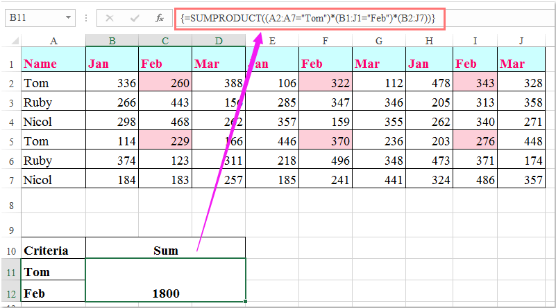
Note:上記の式では: トム & 2月 に基づく列と行の基準は、 A2:A7, B1:J1 列ヘッダーと行ヘッダーには基準が含まれていますが、 B2:J7 合計するデータ範囲です。

最高のオフィス生産性向上ツール

🤖 Kutools AI アシスタント: 以下に基づいてデータ分析に革命をもたらします。 インテリジェントな実行   |  コードを生成  |  カスタム数式の作成  |  データを分析してグラフを生成する  |  Kutools関数を呼び出す...
人気の機能: 重複を検索、強調表示、または識別する   |  空白行を削除する   |  データを失わずに列またはセルを結合する   |   数式なしのラウンド ...
スーパールックアップ: 複数の基準の VLookup    複数の値の VLookup  |   複数のシートにわたる VLookup   |   ファジールックアップ ....
詳細ドロップダウン リスト: ドロップダウンリストを素早く作成する   |  依存関係のドロップダウン リスト   |  複数選択のドロップダウンリスト ....
列マネージャー: 特定の数の列を追加する  |  列の移動  |  Toggle 非表示列の表示ステータス  |  範囲と列の比較 ...
注目の機能: グリッドフォーカス   |  デザインビュー   |   ビッグフォーミュラバー    ワークブックとシートマネージャー   |  リソースライブラリ (自動テキスト)   |  日付ピッカー   |  ワークシートを組み合わせる   |  セルの暗号化/復号化    リストごとにメールを送信する   |  スーパーフィルター   |   特殊フィルター (太字/斜体/取り消し線をフィルター...) ...
上位 15 のツールセット12 テキスト ツール (テキストを追加, 文字を削除する、...)   |   50+ チャート 種類 (ガントチャート、...)   |   40+ 実用的 (誕生日に基づいて年齢を計算する、...)   |   19 挿入 ツール (QRコードを挿入, パスから画像を挿入、...)   |   12 変換 ツール (数字から言葉へ, 通貨の換算、...)   |   7 マージ&スプリット ツール (高度な結合行, 分割セル、...)   |   ... もっと

Kutools for Excel で Excel スキルを強化し、これまでにない効率を体験してください。 Kutools for Excelは、生産性を向上させ、時間を節約するための300以上の高度な機能を提供します。  最も必要な機能を入手するにはここをクリックしてください...

説明


Officeタブは、タブ付きのインターフェイスをOfficeにもたらし、作​​業をはるかに簡単にします

  • Word、Excel、PowerPointでタブ付きの編集と読み取りを有効にする、パブリッシャー、アクセス、Visioおよびプロジェクト。
  • 新しいウィンドウではなく、同じウィンドウの新しいタブで複数のドキュメントを開いて作成します。
  • 生産性を 50% 向上させ、毎日何百回もマウス クリックを減らすことができます!
Comments (17)
No ratings yet. Be the first to rate!
This comment was minimized by the moderator on the site
Brilliant!

The function =SUM(IF(B1:J1="Feb",IF(A2:A7="Tom",B2:J7))) is a great X & Y summation tool.
I would not have thought this logic out on my own.
In fact i took me a minute to deconstruction the operations.

Thank you
This comment was minimized by the moderator on the site
My data that I am trying to retrieve is in a table. Would this impact the result at all? I have:

=SUM(IF('[Primary Controller Active Project Database (KC notes)1.xlsx]Active Project Tracking'!$B2:$B66=X2,IF('[Primary Controller Active Project Database (KC notes)1.xlsx]Active Project Tracking'!$A1:$AV1=AH10,'[Primary Controller Active Project Database (KC notes)1.xlsx]Active Project Tracking'!$H$2:$AV$66)))

So I think the equivalent would be if you did your information above, but in a table in a different workbook. Thoughts?
This comment was minimized by the moderator on the site
If there were negatives in the matrix and you only wanted to include the positives, what would you do? 
I tried to do something like this:

=SUMPRODUCT((Column = Criteria)* ( Row = Criteria) * (second column = Criteria) * (Matrix) * (Matrix >0))

This comment was minimized by the moderator on the site
Is there a way to do this but instead of writing "Tom" & "Feb" in the formula, you are able to reference the criteria cells e.g.A11 & A12?
This comment was minimized by the moderator on the site
Hello, Rianna,Yest, as you said, you can use the cell references to replace the text in the formula, such as:
=SUMPRODUCT((A2:A7=A2)*(B1:J1=C1)*(B2:J7))
=SUM(IF(B1:J1=C1,IF(A2:A7=A2,B2:J7)))
This comment was minimized by the moderator on the site
In the above example which formula should I use if I wanted calculate the sum of the amounts earned by Tom Ruby & Nicol in March?
This comment was minimized by the moderator on the site
Hello, Nabar,To get the result you want, please apply the below formula:=SUMPRODUCT(((A2:A7="Tom")+(A2:A7="Nicol")+(A2:A7="Ruby"))*(B1:J1="Mar")*(B2:J7))
Please try, hope it can help you!
This comment was minimized by the moderator on the site
Hello Skyyang,
Thank you for your response. I tried the formula you suggested but I am not getting the right answer. Probably I wasn't able to put my query correctly. Let me try again I have a spreadsheet with data with daily calculation, I have numbered the first row 1,2,3,4.....132. 2nd, 3rd 4th &5th rows has table headings. The first column has line no's numbered 1, 2,3,.....3005 starting from row 6,range B6:EF3005 has data filled in on everyday basis. In second sheet i have a table in which I want to apply a formula which will look up two line numbers fed in two different rows and calculate the sum from the range B6: EF3005 from the data spreadsheet between the two line numbers from a certain column viz sum of values in column 15 between rows (line No's) 50 & 85.
This comment was minimized by the moderator on the site
Is there a way to make this work with wildcard characters? I'd like to use it on everything starting with certain characters, but with (a fixed number of) undefined characters at the end, i.e. =SUM(IF(B1:J1="Fe*",IF(A2:A7="To*",B2:J7)))
This comment was minimized by the moderator on the site
Should anyone have the same question, this is how I solved it (in Google Sheets, not tested in Excel):

=ArrayFormula(SUM(IF(regexmatch(O5:W5,"^Fe."),IF(regexmatch(N6:N11,"^To."),O6:W11))))

Note that the IF function does not support wildcard characters and that for regexmatch the wildcards are different and can be found here: https://github.com/google/re2/blob/master/doc/syntax.txt
In this particular instance, I used ^ to indicate that Fe & Tom occur at the beginning of text and . to allow for any following character (* would mean zero or more of the previous character, e.g. Fe* would only look for instances with 1 or more "e"s after F)
This comment was minimized by the moderator on the site
I tried to create a formula to calculate if the D12 is blank, it will calculate from K12 to AH12 but it seems this part ' regexmatch(D12,"")' is not working
ArrayFormula(SUM(IF(regexmatch(D12,""),K12:AH12)))
This comment was minimized by the moderator on the site
Thank you so much! You made my day!! @TeSageDS
This comment was minimized by the moderator on the site
how would you do this same formula if you wanted to sum both Feb and March together? please help! thanks

=SUMPRODUCT((A2:A7="Tom")*(B1:J1="Feb")*(B2:J7))
This comment was minimized by the moderator on the site
Hello,Angela,
To solve your problem, you just need to apply the below formula, please try it.

=SUMPRODUCT((A2:A7="Tom")*((B1:J1="Feb")+(B1:J1="Mar"))*(B2:J7)).

Hope it can help you!
This comment was minimized by the moderator on the site
Brilliant
This comment was minimized by the moderator on the site
Worth pointing out that of the two formulas provided above you do not need to enter the SUMPRODUCT formula with Ctrl + Shift + Enter. It will work perfectly well without it.
This comment was minimized by the moderator on the site
Awesome, this is the one what i was looking for. thanks for the help
There are no comments posted here yet
Please leave your comments in English
Posting as Guest
×
Rate this post:
0   Characters
Suggested Locations