メインコンテンツへスキップ

Googleスプレッドシートで依存ドロップダウンリストを作成するにはどうすればよいですか?

著者:シャオヤン 最終更新日:2020年11月25日

Googleシートに通常のドロップダウンリストを挿入するのは簡単な作業かもしれませんが、場合によっては、最初のドロップダウンリストの選択に応じてXNUMX番目のドロップダウンリストを意味する依存ドロップダウンリストを挿入する必要があります。 Googleスプレッドシートでこのタスクにどのように対処できますか?

Googleシートに依存するドロップダウンリストを作成する


Googleシートに依存するドロップダウンリストを作成する

次の手順は、依存するドロップダウンリストを挿入するのに役立つ場合があります。次のようにしてください。

1。 まず、基本的なドロップダウンリストを挿入する必要があります。最初のドロップダウンリストを配置するセルを選択して、[ 且つ > データ検証、スクリーンショットを参照してください:

2。 飛び出した データ検証 ダイアログボックスで 範囲からのリスト 横のドロップダウンリストから 基準 セクションをクリックし、をクリックします ボタンをクリックして、最初のドロップダウンリストを作成するセル値を選択します。スクリーンショットを参照してください。

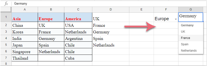
3。 次に、をクリックします Save ボタンをクリックすると、最初のドロップダウンリストが作成されました。 作成したドロップダウンリストからXNUMXつの項目を選択し、次の式を入力します。 =arrayformula(if(F1=A1,A2:A7,if(F1=B1,B2:B6,if(F1=C1,C2:C7,"")))) データ列に隣接する空白のセルに入力し、を押します 入力します キーを押すと、最初のドロップダウンリストアイテムに基づくすべての一致する値が一度に表示されます。スクリーンショットを参照してください。

Note:上記の式では: F1 最初のドロップダウンリストセルです。 A1, B1 & C1 最初のドロップダウンリストの項目は、 A2:A7, B2:B6 & C2:C7 XNUMX番目のドロップダウンリストが基づくセル値です。 あなたはそれらをあなた自身のものに変えることができます。

4。 次に、XNUMX番目の従属ドロップダウンリストを作成し、XNUMX番目のドロップダウンリストを配置するセルをクリックして、[ 且つ > データ検証 データ検証 ダイアログボックスで、 範囲からのリスト 横のドロップダウンから 基準 セクションをクリックし、ボタンをクリックして、最初のドロップダウンアイテムの一致する結果である数式セルを選択します。スクリーンショットを参照してください。

5。 最後に、[保存]ボタンをクリックすると、次のスクリーンショットに示すように、XNUMX番目の依存ドロップダウンリストが正常に作成されました。

最高のオフィス生産性向上ツール

🤖 Kutools AI アシスタント: 以下に基づいてデータ分析に革命をもたらします。 インテリジェントな実行   |  コードを生成  |  カスタム数式の作成  |  データを分析してグラフを生成する  |  Kutools関数を呼び出す...
人気の機能: 重複を検索、強調表示、または識別する   |  空白行を削除する   |  データを失わずに列またはセルを結合する   |   数式なしのラウンド ...
スーパールックアップ: 複数の基準の VLookup    複数の値の VLookup  |   複数のシートにわたる VLookup   |   ファジールックアップ ....
詳細ドロップダウン リスト: ドロップダウンリストを素早く作成する   |  依存関係のドロップダウン リスト   |  複数選択のドロップダウンリスト ....
列マネージャー: 特定の数の列を追加する  |  列の移動  |  Toggle 非表示列の表示ステータス  |  範囲と列の比較 ...
注目の機能: グリッドフォーカス   |  デザインビュー   |   ビッグフォーミュラバー    ワークブックとシートマネージャー   |  リソースライブラリ (自動テキスト)   |  日付ピッカー   |  ワークシートを組み合わせる   |  セルの暗号化/復号化    リストごとにメールを送信する   |  スーパーフィルター   |   特殊フィルター (太字/斜体/取り消し線をフィルター...) ...
上位 15 のツールセット12 テキスト ツール (テキストを追加, 文字を削除する、...)   |   50+ チャート 種類 (ガントチャート、...)   |   40+ 実用的 (誕生日に基づいて年齢を計算する、...)   |   19 挿入 ツール (QRコードを挿入, パスから画像を挿入、...)   |   12 変換 ツール (数字から言葉へ, 通貨の換算、...)   |   7 マージ&スプリット ツール (高度な結合行, 分割セル、...)   |   ... もっと

Kutools for Excel で Excel スキルを強化し、これまでにない効率を体験してください。 Kutools for Excelは、生産性を向上させ、時間を節約するための300以上の高度な機能を提供します。  最も必要な機能を入手するにはここをクリックしてください...

説明


Officeタブは、タブ付きのインターフェイスをOfficeにもたらし、作​​業をはるかに簡単にします

  • Word、Excel、PowerPointでタブ付きの編集と読み取りを有効にする、パブリッシャー、アクセス、Visioおよびプロジェクト。
  • 新しいウィンドウではなく、同じウィンドウの新しいタブで複数のドキュメントを開いて作成します。
  • 生産性を 50% 向上させ、毎日何百回もマウス クリックを減らすことができます!
Comments (18)
No ratings yet. Be the first to rate!
This comment was minimized by the moderator on the site
Hi there. Its been working but for it only appears that only one cell can be formulated.I need help 
For example: in Cell A1, it shows dependent dropdown, but when in cell a2 it does not work.
Thas what help that i need, From A:A, They have all different selection from the dropdown list. Thanks.
This comment was minimized by the moderator on the site
Would it been possible to create pull down menu based of formula?
I use formula "=SUMIFS(Items!$I:$I,Items!$A:$A,K$1,Items!$D:$D,$D2)" (=for example 150) to find the qty on pallet based on item and container size.
So I wanted to create pull down menu like qty 1 pallet, qty 2 pallets, qty 3 pallets,.....
Then user will always order qty of full pallets like 150, 2 x 150, 3 x150, up to 21 x 150.
This comment was minimized by the moderator on the site
Hi, I already created a drop down list like this one, what I'd like to know is how i can, when clicking on one option from that list, restrict what appears as options on another cell. For example, in one cell i can choose between laparoscopy and orthopaedics. If I choose orthopaedics then, the other cell which has a list of doctors, should only show the doctors for orthopedy and not all of them. Does anyone know how to do this?
This comment was minimized by the moderator on the site
Hii Sir,
I Want to Create A Dependent Drop Down List Like
- State(A1):- District(B1):- Taluka(C1) :- Then Information(D1) ,
So I need your Help .
Tell How do you do this Type of Dependent Drop down List in Excel or Google Sheet
This comment was minimized by the moderator on the site
Hi, Shelate,
Maybe the below article can solve your problem, please view it:
https://www.extendoffice.com/documents/excel/5852-excel-multiple-level-drop-down-list.html

Please try, hope it can help you!
This comment was minimized by the moderator on the site
Now is needed to use: =arrayformula(if(F1=A1;A2:A7;if(F1=B1;B2:B6;if(F1=C1;C2:C7;""))))
This comment was minimized by the moderator on the site
Thank you soooo much!
This comment was minimized by the moderator on the site
Hi,
I was wondering if anyone could advise me with this? I've followed the above steps but on step 3 rather than getting:
"...all the matching values based on the first drop down list item have been displayed at once," I am just seeing one value (the top one from the drop down list).
My cells are placed slightly differently and the first drop down is filled from another sheet (from anywhere int eh column excluding the top row) so my formula is:

=arrayformula(if(VLE!D2:D=B11,B12,if(VLE!D2:D=C11,C12:C14,if(VLE!D2:D=D11,D12:D14,if(VLE!D2:D=E11,E12:E16,if(VLE!D2:D=F11,F12:F16,""))))))

It is correctly displaying the top drop down option for each of (using cell numbers from the step 3 example on this page) A1, B1, and C1 so, again using this page's example, if I select Asia form the F1 drop down, I would get China, but nothing further


Any suggestions?

Many thanks! Nick
This comment was minimized by the moderator on the site
If the first drop own is on sheet 1 A1, will this work were I want the second drop down as sheet 1 A2, but to have its data range on a separate sheet?
This comment was minimized by the moderator on the site
Ich bekomm immer die Meldung "Fehler beim Parsen der Formel" wenn ich =arrayformula(if(F1=A1,A2:A7,if(F1=B1,B2:B6,if(F1=C1,C2:C7,"")))) eingebe. Was ist der "Weiter-Schlüsel"? Reicht es nicht wie bei Excel die Formel einzugeben?
This comment was minimized by the moderator on the site
Ersetzen Sie den , zu ;
es hat für mich funktioniert
This comment was minimized by the moderator on the site
This is the best explanation I have found, so thank you for that!

In my situation, I am working with over 200 rows with more being continuously added. Is there an easier/more efficient way to handle this many rows?
This comment was minimized by the moderator on the site
Yes, if you don't put number index to specify ending cell.
Like instead of C2:C7 you put C2:C. This will automatically tell the array formula, that you want to consider all values in column "C" starting at "C2".
This comment was minimized by the moderator on the site
What happens if I want exactly the same dropdown list in F2 as you have in F1 ?
I tried, and it doesn't overwrite D1:D7 .. meaning D1:D7 is only available once.
I need something else, double dropdown, but on many-many lines .. guess I must use another system then .. not sure which ..
This comment was minimized by the moderator on the site
Hi, Xained,
This method can only applied to one cell, if you have some good ways for applying this to multiple cells, please comment here.

Thank you!
This comment was minimized by the moderator on the site
Please, guide me how to do that.Thanks
This comment was minimized by the moderator on the site
혹시, 하나의 셀이 아닌 여러셀에 할 수 있는 방법을 알 수 있을까요?
This comment was minimized by the moderator on the site
내말이... 시바 좃빠지게 따라했디만 밑에줄은 안되노..
There are no comments posted here yet
Please leave your comments in English
Posting as Guest
×
Rate this post:
0   Characters
Suggested Locations