ExcelのXNUMXつのセルに複数の値を返すようにvlookupする方法は?
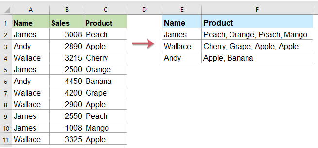
通常、Excelでは、VLOOKUP関数を使用するときに、条件に一致する値が複数ある場合は、最初の値を取得できます。 しかし、次のスクリーンショットのように、基準を満たすすべての対応する値をXNUMXつのセルに返したい場合があります。どうすれば解決できますか?
TEXTJOIN関数を使用して複数の値を2019つのセルに返すVlookup(Excel365およびOfficeXNUMX)
ユーザー定義関数を使用して複数の値をXNUMXつのセルに返すVlookup
便利な機能を備えたXNUMXつのセルに複数の値を返すVlookup
TEXTJOIN関数を使用して複数の値を2019つのセルに返すVlookup(Excel365およびOfficeXNUMX)
Excel2019やOffice365などの上位バージョンのExcelを使用している場合は、新しい機能があります- テキスト結合、この強力な関数を使用すると、一致するすべての値をすばやくvlookupしてXNUMXつのセルに返すことができます。
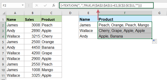
一致するすべての値をXNUMXつのセルに返すVlookup
結果を入力する空白のセルに次の数式を適用して、を押してください Ctrl + Shift + Enter キーを一緒に押して最初の結果を取得し、塗りつぶしハンドルをこの数式を使用するセルまでドラッグすると、以下のスクリーンショットに示すように、対応するすべての値が取得されます。
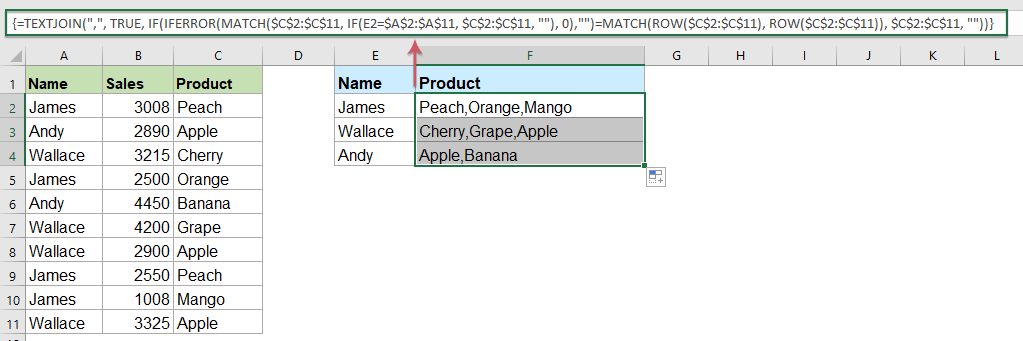
重複することなくすべての一致する値をXNUMXつのセルに返すVlookup
重複することなくルックアップデータに基づいて一致するすべての値を返したい場合は、次の式が役立つ場合があります。
次の数式をコピーして空白のセルに貼り付け、を押してください Ctrl + Shift + Enter キーを合わせて最初の結果を取得し、この数式をコピーして他のセルに入力すると、以下のスクリーンショットに示すように、重複する値なしで対応するすべての値が取得されます。
ユーザー定義関数を使用して複数の値をXNUMXつのセルに返すVlookup
上記のTEXTJOIN関数は、Excel2019およびOffice365でのみ使用できます。他の下位バージョンのExcelを使用している場合は、このタスクを完了するためにいくつかのコードを使用する必要があります。
一致するすべての値をXNUMXつのセルに返すVlookup
1。 を押し続けます Alt + F11 キー、そしてそれは開きます アプリケーション向け Microsoft Visual Basic 窓。
2に設定します。 OK をクリックします。 インセット > モジュール、次のコードをに貼り付けます モジュールウィンドウ.
VBAコード:XNUMXつのセルに複数の値を返すVlookup
Function ConcatenateIf(CriteriaRange As Range, Condition As Variant, ConcatenateRange As Range, Optional Separator As String = ",") As Variant
'Updateby Extendoffice
Dim xResult As String
On Error Resume Next
If CriteriaRange.Count <> ConcatenateRange.Count Then
    ConcatenateIf = CVErr(xlErrRef)
    Exit Function
End If
For i = 1 To CriteriaRange.Count
    If CriteriaRange.Cells(i).Value = Condition Then
        xResult = xResult & Separator & ConcatenateRange.Cells(i).Value
    End If
Next i
If xResult <> "" Then
    xResult = VBA.Mid(xResult, VBA.Len(Separator) + 1)
End If
ConcatenateIf = xResult
Exit Function
End Function
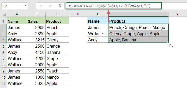
3。 次に、このコードを保存して閉じ、ワークシートに戻って、次の数式を入力します。 =CONCATENATEIF($A$2:$A$11, E2, $C$2:$C$11, ", ") 結果を配置する特定の空白のセルに移動し、塗りつぶしハンドルを下にドラッグして、必要なXNUMXつのセルに対応するすべての値を取得します。スクリーンショットを参照してください。
重複することなくすべての一致する値をXNUMXつのセルに返すVlookup
返される一致する値の重複を無視するには、以下のコードを使用してください。
1。 を押し続けます Altキー+ F11 キーを押して アプリケーション向け Microsoft Visual Basic 窓。
2に設定します。 OK をクリックします。 インセット > モジュール、次のコードをに貼り付けます モジュールウィンドウ.
VBAコード:Vlookupを実行し、複数の一意の一致値をXNUMXつのセルに返します
Function MultipleLookupNoRept(Lookupvalue As String, LookupRange As Range, ColumnNumber As Integer)
'Updateby Extendoffice
    Dim xDic As New Dictionary
    Dim xRows As Long
    Dim xStr As String
    Dim i As Long
    On Error Resume Next
    xRows = LookupRange.Rows.Count
    For i = 1 To xRows
        If LookupRange.Columns(1).Cells(i).Value = Lookupvalue Then
            xDic.Add LookupRange.Columns(ColumnNumber).Cells(i).Value, ""
        End If
    Next
    xStr = ""
    MultipleLookupNoRept = xStr
    If xDic.Count > 0 Then
        For i = 0 To xDic.Count - 1
            xStr = xStr & xDic.Keys(i) & ","
        Next
        MultipleLookupNoRept = Left(xStr, Len(xStr) - 1)
    End If
End Function
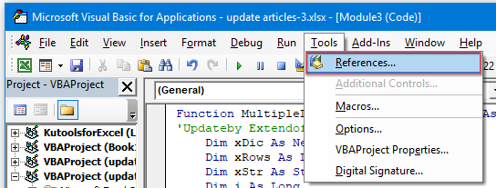
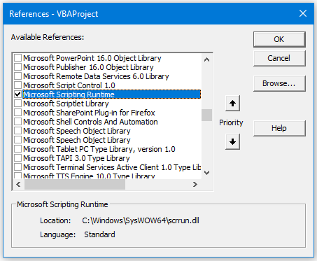
3。 コードを挿入したら、をクリックします ツール > 参考文献 オープンで アプリケーション向け Microsoft Visual Basic ウィンドウ、そして、ポップアウトで 参照– VBAProject ダイアログボックス、チェック Microsoftスクリプトランタイム 内のオプション 利用可能な参考文献 リストボックス、スクリーンショットを参照してください:
 |
 |
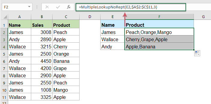
4。 次に、をクリックします OK ダイアログボックスを閉じるには、コードウィンドウを保存して閉じ、ワークシートに戻り、次の式を入力します。 =MultipleLookupNoRept(E2,$A$2:$C$11,3) into a blank cell where you want to output the result, and then drag the fill hanlde down to get all matching values, see screenshot:
便利な機能を備えたXNUMXつのセルに複数の値を返すVlookup
あなたが私たちを持っているなら Kutools for Excelそのと 高度な結合行 この機能を使用すると、同じ値に基づいて行をすばやくマージまたは結合し、必要に応じていくつかの計算を実行できます。
インストールした後 Kutools for Excel、次のようにしてください。
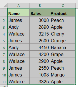
1。 別の列に基づいてXNUMXつの列データを結合するデータ範囲を選択します。
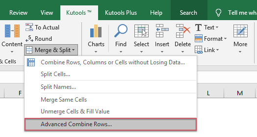
2に設定します。 OK をクリックします。 クツール > マージ&スプリット > 高度な結合行、スクリーンショットを参照してください:
3。 飛び出した 高度な結合行 ダイアログボックス:
- 結合するキー列名をクリックしてから、 主キー
- 次に、キー列に基づいてデータを結合する別の列をクリックし、をクリックします。 組み合わせる 結合されたデータを分離するためにXNUMXつのセパレータを選択します。
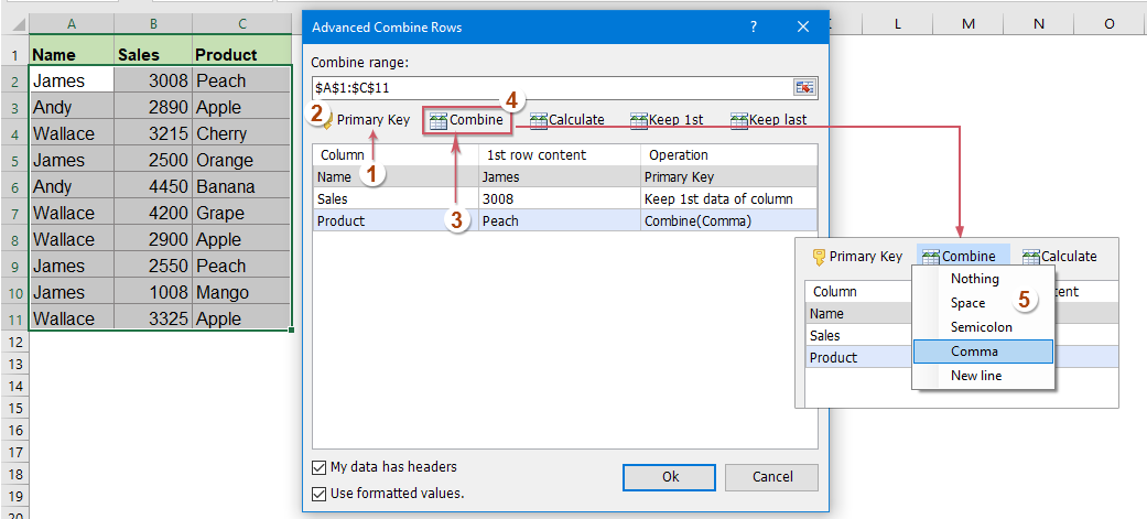
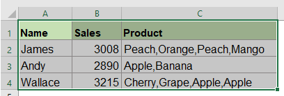
4. 次に、をクリックします。 OK ボタンをクリックすると、次の結果が得られます。
 |
 |
今すぐExcel用のKutoolsをダウンロードして無料トライアル!
より相対的な記事:
- いくつかの基本的な例と高度な例を含むVLOOKUP関数
- Excelでは、VLOOKUP関数はほとんどのExcelユーザーにとって強力な関数であり、データ範囲の左端の値を検索し、指定した列から同じ行の一致する値を返すために使用されます。 このチュートリアルでは、Excelのいくつかの基本的な例と高度な例でVLOOKUP関数を使用する方法について説明します。
- XNUMXつまたは複数の基準に基づいて複数の一致する値を返します
- 通常、VLOOKUP関数を使用すると、特定の値を検索して一致するアイテムを返すのは簡単です。 しかし、XNUMXつ以上の基準に基づいて複数の一致する値を返そうとしたことがありますか? この記事では、Excelでこの複雑なタスクを解決するためのいくつかの式を紹介します。
- Vlookupと複数の値を垂直方向に返す
- 通常、Vlookup関数を使用して最初の対応する値を取得できますが、特定の基準に基づいて一致するすべてのレコードを返したい場合もあります。 この記事では、vlookupして、一致するすべての値を垂直方向、水平方向、またはXNUMXつのセルに返す方法について説明します。
- Vlookupとドロップダウンリストから複数の値を返す
- Excelで、ドロップダウンリストから複数の対応する値をvlookupして返すにはどうすればよいですか。つまり、ドロップダウンリストからXNUMXつの項目を選択すると、そのすべての相対値が一度に表示されます。 この記事では、ソリューションを段階的に紹介します。
最高のオフィス生産性向上ツール
| 🤖 | Kutools AI アシスタント: 以下に基づいてデータ分析に革命をもたらします。 インテリジェントな実行 | コードを生成 | カスタム数式の作成 | データを分析してグラフを生成する | Kutools関数を呼び出す... |
| 人気の機能: 重複を検索、強調表示、または識別する | 空白行を削除する | データを失わずに列またはセルを結合する | 数式なしのラウンド ... | |
| スーパールックアップ: 複数の基準の VLookup | 複数の値の VLookup | 複数のシートにわたる VLookup | ファジールックアップ .... | |
| 詳細ドロップダウン リスト: ドロップダウンリストを素早く作成する | 依存関係のドロップダウン リスト | 複数選択のドロップダウンリスト .... | |
| 列マネージャー: 特定の数の列を追加する | 列の移動 | Toggle 非表示列の表示ステータス | 範囲と列の比較 ... | |
| 注目の機能: グリッドフォーカス | デザインビュー | ビッグフォーミュラバー | ワークブックとシートマネージャー | リソースライブラリ (自動テキスト) | 日付ピッカー | ワークシートを組み合わせる | セルの暗号化/復号化 | リストごとにメールを送信する | スーパーフィルター | 特殊フィルター (太字/斜体/取り消し線をフィルター...) ... | |
| 上位 15 のツールセット: 12 テキスト ツール (テキストを追加, 文字を削除する、...) | 50+ チャート 種類 (ガントチャート、...) | 40+ 実用的 式 (誕生日に基づいて年齢を計算する、...) | 19 挿入 ツール (QRコードを挿入, パスから画像を挿入、...) | 12 変換 ツール (数字から言葉へ, 通貨の換算、...) | 7 マージ&スプリット ツール (高度な結合行, 分割セル、...) | ... もっと |
Kutools for Excel で Excel スキルを強化し、これまでにない効率を体験してください。 Kutools for Excelは、生産性を向上させ、時間を節約するための300以上の高度な機能を提供します。 最も必要な機能を入手するにはここをクリックしてください...
")
Officeタブは、タブ付きのインターフェイスをOfficeにもたらし、作業をはるかに簡単にします
- Word、Excel、PowerPointでタブ付きの編集と読み取りを有効にする、パブリッシャー、アクセス、Visioおよびプロジェクト。
- 新しいウィンドウではなく、同じウィンドウの新しいタブで複数のドキュメントを開いて作成します。
- 生産性を 50% 向上させ、毎日何百回もマウス クリックを減らすことができます!
")